Wednesday, March 1, 2017

Data Analyst ND 2, data wrangling, SQL

Data Wrangling

Shanon Bradshaw, director of education at MongoDB, open source NoSQL database.
Data scientist spend 70% time on data wrangling. If you don’t take the time to ensure your data is in good shape before doing any analysis, you run a big risk of wasting a lot of time later on, or losing the faith of your colleagues who depend on your data.
Generally, we should not trust any data we get.where does it come from? typo, missing value, different format of daytime, outliers.

Data extraction

Extracting data from CSV, excel and local/remote JSON files are relatively easy. See python codes here

Read XML/HTML

XML design goals:
  • platform-independent data transfer
  • easy to write code to read/write
  • document validation
  • human readable
  • support a wide variety of applications
  • robust parsers in most languages.
It is very common to fill in the form to make HTML request to get desirable information. what exact information do you send in the post request can be seen in the browser developer tool -> Network -> Data_Elements.aspx?Data=2 -> Headers -> Form Data. there are 7 parameters you need to pass the form.
python codes here and practise
simple comparison:
Difference XML HTML
brith 1996 1993
pre-defined tag? NO Yes
purpose store data display data
? Markup Language Extensible HyperText

Data Quality

This process is very situation specific.
  • typo
  • legacy data
  • time format
  • statistical analysis, identify causes

SQL

The major content is similar to the free course: intro to Relational Databases. I actually wrote a blog post last August when I was at stage 5( back end ) of the Intro to Programming ND.
The nice improvement made by the nanodegree program is a set up of the local environment and a set of problems to get you play with the chinook database.

comparison of different RDBMS

SQL environments:
  • mysql,postgresql,oracle: code->network-> server-> data on disk
  • sqlite: code-> DB library-> data on disk
born creator features DB-API
sqlite 2000 D. Richard Hipp fast, free sqlite3
SQL Server 1989 Microsoft SaaS
MySQL 1995 Oracle partial free mysql.connector
PostgreSQL 1996 UC berkeley more format, free psycopg2
I am touched by the SQLite author, Hipp, who keep it free to everyone
“It’s very clear to me that if I’d had any business sense whatsoever I could have made a lot of money, but I don’t,” he says. “I like to tell people that we make enough to live fine in Charlotte, North Carolina. We don’t make nearly enough money to live in London or San Francisco, but we don’t live there so that’s OK,” he adds - with a touch, just a touch, of wistfulness.

sqlite

SQLite is preinstalled in Mac. My version is 3.13, while the latest version is 3.17. I haven’t figured out a simple way to update it. sqlite3 in the shell to enter the environment.
.open chinook.db
.exit
.quit
.help
.tables
.schema
Alternatively, sqlite studio is a visual appealing IDE. You can see how many tables, which is the primary key and the whole tabular data at your clicks. No black box anymore. it really makes life much easier. I guess the only catch is to be careful about the size. Get a sample size first.

sqlite datatype

  • TEXT
  • REAL
  • INTEGER
  • BLOB
  • NULL
no class for storing data/time, TEXT or NUMERIC can be used to store data. There are built-in function to parse into the right format

sqlite tricks

change output format
.show # show setting
.mode list  # default output mode, default separator is a pipe symbol
.separator ","
.mode quote
.mode line
.mode column
.mode tabs
.header off
.mode insert  # used to input data elsewhere
check, output results
.tables  # see a list of tables
.schema
.databases
.output filename.txt # all subsequent results will be written to this file
import/ output table
.mode csv  # alignment format
.import somedata.csv table1 # import table

.header on
.mode csv
.once filename.csv
select * from table1;
.sytem open filename.csv  # open file to display
create a new SQLite database:
sqlite3 ex1 # enter sqlite and create exl database
create table tb1(one varchar(10), two smallint);
insert into tb1 values('hello!',10);
insert into tb1 values('goodbye', 20);
CREATE TABLE tb2 (f1 varchar(30) primary key,
f2 text,f3 real);
note: SQL qury command is not case-sensitive. But the “text” value is case-sensitive.

chinook database

The sample database at your disposal is called chinook, hosted at https://chinookdatabase.codeplex.com/. The Chinook data model represents a digital media store, including 11 tables (artists, albums, media tracks, invoices and customers). It was first public in 2008. Now it is available for all major languages.
chinook data model
example query
.open chinook.db
SELECT Name FROM Track WHERE Composer='AC/DC';
SELECT Composer, sum(Milliseconds) FROM Track WHERE Composer='Johann Sebastian Bach';
SELECT FirstName, LastName, Title, Birthdate FROM Employee;
SELECT Composer, Name FROM Track WHERE Composer = 'Stevie Ray Vaughan';
select composer, count(*) from track group by composer  order by count(*) desc limit 10;
select artist.name, album.title from album join artist on artist.artistid = album.artistid where name = 'Iron Maiden' or name = 'Amy Windhouse';
select billingcountry, count(*) from invoice group by billingcountry order by count(*) desc limit 3;
select customer.email, customer.firstname,customer.lastname, sum(invoice.total) from customer, invoice on customer.customerid = invoice.customerid group by invoice.customerid order by sum(invoice.total) desc limit 1;
select customer.email, customer.firstname, customer.lastname, genre.name from customer, invoice, invoiceline, track,genre on customer.customerid = invoice.customerid
select customer.email, customer.firstname, customer.lastname, genre.name from customer, invoice, invoiceline, track,genre on customer.customerid = invoice.customerid and invoice.invoiceid = invoiceline.invoiceid and invoiceline.trackid = track.trackid and track.genreid = genre.genreid where genre.name="Rock" group by customer.email;
select billingcity, sum(Total) from invoice group by billingcity order by sum(total) desc limit 10;
select billingcity,count(Genre.Name),genre.name from invoice, invoiceline,track, genre on invoice.invoiceid= invoiceline.invoiceid and invoiceline.trackid = track.trackid and track.genreid = genre.genreid group by billingcity order by sum(Invoice.total) desc limit 3;

For Big-Data Scientists, ‘Janitor Work’ Is Key Hurdle to Insights

Yet far too much handcrafted work — what data scientists call “data wrangling,” “data munging” and “data janitor work” — is still required. Data scientists, according to interviews and expert estimates, spend from 50 percent to 80 percent of their time mired in this more mundane labor of collecting and preparing unruly digital data, before it can be explored for useful nuggets.
Several start-ups are trying to break through these big data bottlenecks by developing software to automate the gathering, cleaning, and organizing of disparate data, which is plentiful but messy.
“It’s an absolute myth that you can send an algorithm over raw data and have insights pop up,”
The result, Mr. Weaver said, is being able to see each stage of a business in greater detail than in the past, to tailor product plans and trim inventory. “The more visibility you have, the more intelligent decisions you can make,” he said.
But if the value comes from combining different data sets, so does the headache. Data from sensors, documents, the web and conventional databases all come in different formats. Before a software algorithm can go looking for answers, the data must be cleaned up and converted into a unified form that the algorithm can understand.
Data formats are one challenge, but so is the ambiguity of human language. For example, “drowsiness,” “somnolence” and “sleepiness” are all used. A human would know they mean the same thing, but a software algorithm has to be programmed to make that interpretation. That kind of painstaking work must be repeated, time and again, on data projects.
“You can’t do this manually,” Ms. Shahani-Mulligan said. “You’re never going to find enough data scientists and analysts.”
“You prepared your data for a certain purpose, but then you learn something new, and the purpose changes,” said Cathy O’Neil, a data scientist at the Columbia University Graduate School of Journalism, and co-author, with Rachel Schutt, of “Doing Data Science” (O’Reilly Media, 2013).

Thursday, February 23, 2017

Data Analyst ND 1, Statistics

7-day free trial: 2017-2-22~3.1
Program director: Mat Leonard
content developer: Caroline Buckey

Update on 2017-2-27

I soon found there are so much overlap with my existing knowledge, I can even finish all the projects in the 7-day trial! But I change my goal from getting a nano degree to filling my knowledge gap. I am close to get my first data scientist job, a nanodegree is not so important to me now .
projects recap:
  1. bike share. The main takeaway is how to slice the dataset to smaller size and how to use datetimemodule to parse the timestamp
  2. Stroop effect. hypothesis test, epecially t-test.
  3. Titanic Analysis. get you familar with numpy and pandas. This is the same with stage 5 (choose your path) of Intro to Programming ND.
  4. open street map. focus on data wrangling skills. parse various data types: csv, excel, JSON, XML, HTML. extract data from database, SQL or NoSQL.
  5. (Data Set Options) practise R
  6. Enron Email. This is the same with the free course “Intro to machine learning”
  7. (Data Set Options) the course content is about JavaScript plotting API: D3 and Dimple. And the fancy way to draw world map!
  8. Free trial screener of udacity charged courses. This is the same the free course “A/B testing

P0 Bay Area Bike Share Analysis

Two of the major parts of the data analysis process: data wrangling and exploratory data analysis.
before you even start looking at data, think about some questions you might want to understand about the bike share data.
After all, your best analysis is only as good as your ability to communicate it.
When dealing with a lot of data, it can be useful to start by working with only a sample of the data.

P1: Statistics

The course materials in this section has 11 lessons + placement advisor to help you locate your knowledge gap in case you already know some statistics.
Actually, Udacity has provided 2 free courses:

Staticstics placement Advisor

If you are comfortable:
  • Performing a hypothesis test using a two-sample t-test
  • Calculating a p-value and a confidence interval
  • Deciding whether to reject the null based on the result of the above
continue straight to Project 1.

constructs and their operational definition

constructs are concepts difficult to define and measure. Scientists try to quantify them by attemping their operational definition. units are at the heart of measurement.
  • Memory:
  • Guilt
  • Love
  • Stress: levels of cortisol (the stress hormone)
  • depression: Beck’s Depression Inventory: 21 questions
  • anger: number of profanities uttered per min
  • happiness: ratio of minutes spent simling to minutes not smiling

interpreting scatter plots

We can infer a trend, but it is not necessary true.
Correlation does not imply causation. Golden Arches Theory of conflict prevention: No 2 countries with a McDonald’s have ever gone to war since opening McDonald’s.
  • show relationships: observational study, surveys
  • show causation: controlled experiment. Use double blind to avoid placebo effect (unconsciously or consciously alter the measurement).
Most research studies only use a sample because collecting data about a entire population is way too expensive. As a result, we expect our estimates will not be exactly accurate when we do this.
A fixed number is called constant, a changeable number is called variable.
\bar{x} is for sample mean, \mu is for population mean.
We can make prediction by either correlation or causation.

standard normal distribution

Any normal distribution can be normalized by the z-score: z=\frac{x-\mu}{\sigma}
z-table shows the probality the something is less than a z-score.
standard error(SE) is the standard deviation of the distribution of the sample means. SE= \frac{\sigma}{\sqrt(n)}
This is called central limit theorem.
margin of error: 95% of sample means fall within \frac{2\sigma}{\sqrt(n)}
critical value: 98% of sample means fall within \frac{2.33\sigma}{\sqrt(n)}
The level of unlikely is called alpha levels: 5%, 1%, 0.1%. For one-tailed critical region, these correspod to z-value of 1.65, 2.33, 3.08.
e.g. if z= 1.82, we say \bar x is significant at p <0.05. This is interesting. ==The outlier is statistically significant.==
We can also have two-tailed critical region, similar to

hypothesis

H0(null hypothesis): the mean of intervention is outside the critical region.
Ha(alternative hypthesis): the mean of intervention is inside the critical region.
we can’t prove that the null hypothesis is true. we can only obtain evidence to reject the null hypothesis.
e.g. Most dogs have 4 legs. (significance level = 50%)

t distribution

z-test works when we know mu and sigma, but we don’t.
Degree of freedoms are the number of pieces of information that can be freely varied without violating any given restrictions.They are independent pieces of information available to estimate another piece of information.
sample deviation = \sqrt{\frac{\sum_i (x_i-\bar x)^2}{n-1}}, n-1 is the effective sample size.
t-distribution is kind of a flatterned form of normal distribution. As the degree of freedom tends to infinity, they overlap with each other.
t-value can be obtained by checking t-Table
from sample to calculte the t-value:
def t_value(nums, mean):
  length = len(nums)
  print(length)
  x_bar= np.mean(nums)
  sample_sd = np.sqrt(np.var(a)*length/(length-1))
  t = (x_bar-mean)/sample_sd*np.sqrt(length)
  print('x_bar={0:.2f}\n sample_sd={1:.3f}\n t={2:.3f}'.format(x_bar,sample_sd,t))
def t_value(x_bar,ssd, mean,num):
  print((x_bar-mean)/ssd*np.sqrt(num))
from t-value to get the 2-tailed p-value: Link to GraphPad
One-sample test, dependent samples, repeated measures:
  • two conditions,
  • longitudinal(t1,t2),
  • pretest & posttest
this approach is cheap, but the downside is the carry-on effects: 2nd measurement can be affected by first treatment, and order may influnce results.

types of effect size measue

difference: mean, deviation
correlation
statistical significance doen’t mean important, large, sizeable or meaningful. It means rejected the null, results are not likely due to chance (sampling error).
Cohen’s d measure standardized mean difference.

independent samples

standard deviation s^2 = s1^2 +s2^2
standard error = s/\sqrt n=\sqrt{s_1^2/n1+s_2^2/n2}

Sunday, February 19, 2017

Self-driving Car ND A1, finding lane

I am so excited to enroll in Udacity’s flagship program: self-driving car!
This is term one, which includes 5 projects and 24 lessons (from 2.16 to 5.29):
  • Lane-Finding Project (due 2.25)
  • Traffic Sign Classifier Project (3.27)
  • Behavioral Cloning Project (4.17)
  • Advanced Lane Finding Project(5.1)
  • Vehicle Tracking Project (5.15)
C++ will be used in term 2 and term 3, with topics in sensor fusion and path planning.
For a quick glance, I notice quite a few overlapping contents with other nanodegree programs. As a result of the overlap, so far I already finish 2/3 of the total 24 lessons.
  • 3 lessons are exactly the same from the free udacity course (intro to machine learning) by Sebastian.
  • 5 lessons are career services (resume, link-in, github, interview), pretty much the same with MLND.
  • 7 lessons are deep learning basis. Actually, the original TensorFlow Deep learning by Vincent has just been overhauled.
So after subtracting the obove courses, the pure, authentic lessons that directly teach self-driving car are only 9. Obvious, these courses are never enough to build a self-driving car. These courses are just a window to a new world. Be prepared and actively learn much more!

Available sources

Instructor:
David Silver Princeton graduate in CS (2004), previously worked on automous car at Ford for 3 months.
Ryan Keenan recovering astrophysicist (2007-2015)
By the way, the team in CMU to lead in DARPA Grand Challenge (1st in 2004, 2nd in 2005 due to home-assembled hardware, 1st in 2007) was lead by Whittaker, who has all his degrees in Civil Engineering in 1970s. He said,
If you haven’t done everything, you haven’t done a thing.
Your mentor, Pratheerth Padman, Martijn de Boer
  • Check in with you weekly to make sure that you are on track
  • Help you to set learning goals
  • Guide you to supplementary resources when you get stuck
  • Respond to any questions you have about the program.
Self-driving car is taught by both approaches:
  • Robotics
  • Deep Learning
A free Udacity course, Introduction to Computer Vision.

Setup

Environment setup. The problem is opencv3 only compatible with python 3.5 while the latest python is 3.6. So I build a new env for this project.
conda create --name=car python=3.5 anaconda
pip install pillow
source activate car
conda install -c menpo opencv3=3.1.0
pip install moviepy

python
import imageio
imageio.plugins.ffmpeg.download()
Read a image file has many ways:
  1. scipy.ndimage.imread() # rgb format
  2. matplotlib.image.imread() # rgb format
  3. cv2.imread() # bgr format
Be careful if you use cv2 to read image.

Finding Lane lines

5 region masking

triangle mask
ysize, xsize = image.shape[0:2] # size is (y,x) format
region_select = np.copy(image)
left_bottom = [0, 539] # point is (x,y) format
right_bottom = [900, 300]
apex = [400, 0]

# Fit lines (y=Ax+B) to identify the  3 sided region of interest
# np.polyfit() returns the coefficients [A, B] of the fit
fit_left = np.polyfit((left_bottom[0], apex[0]), (left_bottom[1], apex[1]), 1)
fit_right = np.polyfit((right_bottom[0], apex[0]), (right_bottom[1], apex[1]), 1)
fit_bottom = np.polyfit((left_bottom[0], right_bottom[0]), (left_bottom[1], right_bottom[1]), 1)

# Find the region inside the lines
XX, YY = np.meshgrid(np.arange(0, xsize), np.arange(0, ysize))
region_thresholds = (YY > (XX*fit_left[0] + fit_left[1])) &  (YY > (XX*fit_right[0] + fit_right[1])) & (YY < (XX*fit_bottom[0] + fit_bottom[1]))

# Color pixels red which are inside the region of interest
region_select[region_thresholds] = [255, 0, 0]

10 Canny Edge detection

John F. Canny developed this algorithm in 1986.
# Define a kernel size for Gaussian smoothing / blurring
kernel_size = 5 # Must be an odd number (3, 5, 7...)
blur_gray = cv2.GaussianBlur(gray,(kernel_size, kernel_size),0)
# Define our parameters for Canny and run it
low_threshold = 50
high_threshold = 100
edges = cv2.Canny(blur_gray, low_threshold, high_threshold)

13 Hough Transform

In 1962, Paul Hough devised a method for representing lines in parameter space, which is called Hough space.
y = mx + b
Usually, we use (x,y) space, but Hough space is (m,b) or (\rho, \theta)
# Define the Hough transform parameters
# Make a blank the same size as our image to draw on
rho = 1
theta = np.pi/180
threshold = 1
min_line_length = 10
max_line_gap = 1
line_image = np.zeros_like(image) #creating a blank to draw lines on
# Run Hough on edge detected image
lines = cv2.HoughLinesP(edges, rho, theta, threshold, np.array([]),min_line_length, max_line_gap)
# Iterate over the output "lines" and draw lines on the blank
for line in lines:
    for x1,y1,x2,y2 in line:
        cv2.line(line_image,(x1,y1),(x2,y2),(255,0,0),10)
documentation link:

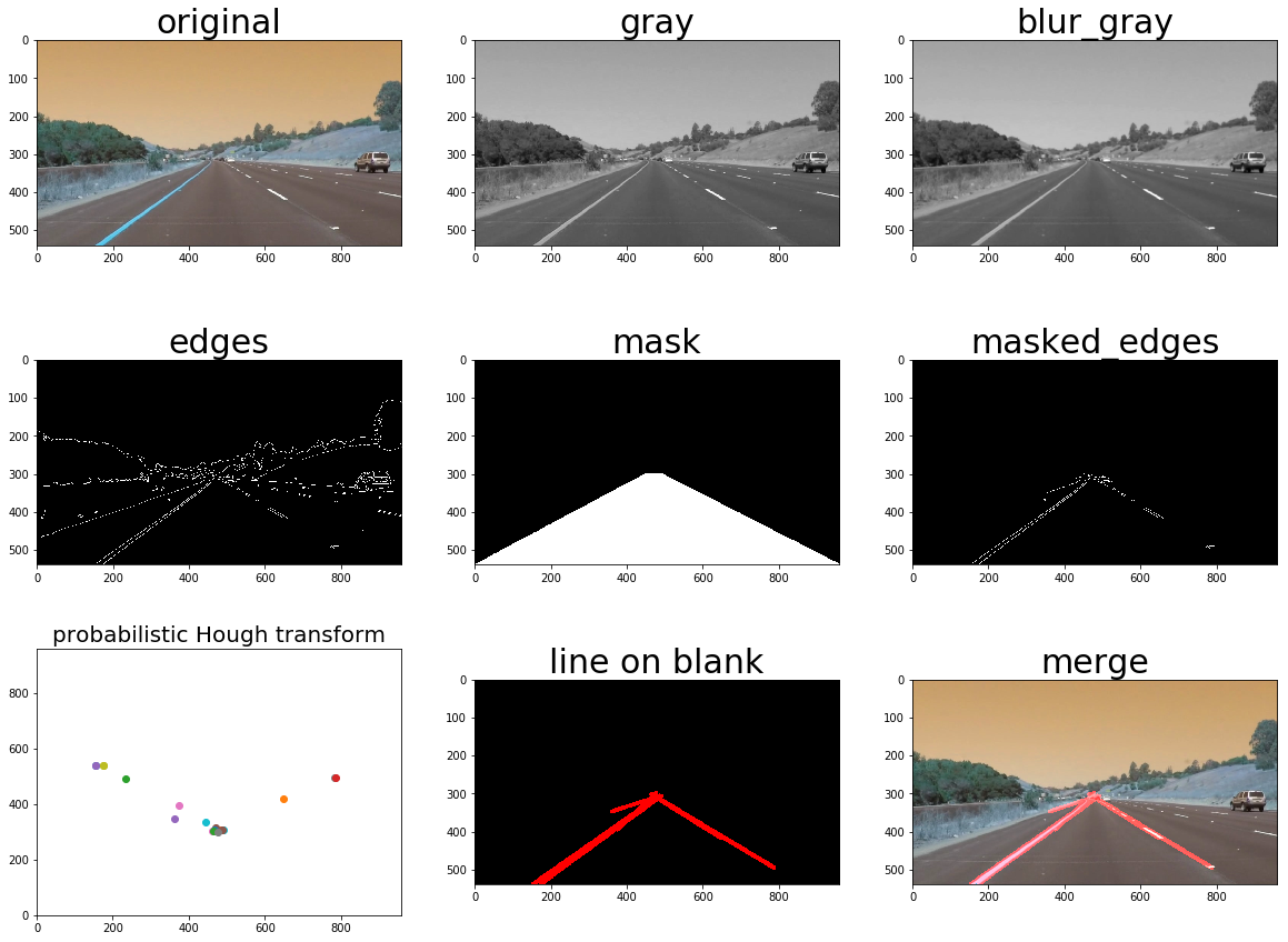
project pipeline

My pipeline consisted of following steps:
step Action code functions
1 convert image file to 3D np array cv2.imread
2 convert image to grayscale cv2.cvtColor
3 smooth image to suppress noise cv2.GaussianBlur
4 get edges by canny’s gradient method cv2.Canny
5 propose a mask region cv2.fillPoly
6 retain masked edges cv2.bitwise_and
7 probalistic hough transform cv2.HoughLinesP
8 draw lines on a blank image cv2.line
9 merge original image with lines cv2.addWeighted
The highlighted part is key steps.
The corresponding result for each step is:
9-photo
Note that the Hough line points are drawn inconsistent with the normal mathematical coordinates.
I used reviewer’s suggestions to tune the parameters of cv2.HoughLinesP() and get much better results. The problem is still false positive. The idea I have is to use a queue to store the point positions that are closest to car (max of y value), and use this to pick the “right points”. Then np.polyfit() the points and plot 2 nice lines.

for video

from moviepy.editor import VideoFileClip
from IPython.display import HTML
white_output = 'white.mp4'
clip1 = VideoFileClip("solidWhiteRight.mp4")
white_clip = clip1.fl_image(process_image) 
%time white_clip.write_videofile(white_output, audio=False)
HTML("""<video width="960" height="540" controls><source src="{0}"></video>""".format(white_output))
where process_image is a user-define function that process a 3-channel image and output an image with lines drawn on.

Friday, February 17, 2017

TensorBoard

On 2017.2.16 at Dev Summit 2007, TensorFlow 1.0 is announced! It has been 15 months since it was open sourced.
Tensorflow is also working on high-level APIs for better user experience. tf.layersis already available but without further detail of how to train.
tf.keras will be available around TensorFlow 1.2.
I love what Lily Peng said about the career-changing:
In a previous life I was a doctor, and I’ve been repurposed as a product manager at google.

how to use Tensorboard

In Dev Summit, Dandelion demonstrated the magic of TensorBoard. The highlighted codes in the slides are very impressive. video, source code and slides
The use of tensorboard is actually 2 steps:
  1. use a tf.summary.FileWriter(folder_name) object to add everything you want to show, which will be stored in a folder in lcoal disk.
  2. In terminal, tensorboard --logdir=folder_name which will output data to something like “0.0.0.0:6006”. Open it in a browser.
So the major work in 1st step. Example code is here.
Several tricks:
  1. use with tf.name_scope() to name a group of tensors or operations.
  2. use name= to name a single tensor
  3. use writer = tf.summary.FileWriter( folder_name)to create writer
  4. use writer.add_graph(sess.graph) to add graph. Note: if you revise the graph, remember to reset it to avoid ghost graph.
  5. use writer.add_summary(scalar/histogram/image tensor,step) to add a point for the plotting data. Each tensor will be wrapped by tf.summary.scalar/histogram/image and evaluated at sees.run step.
  6. tf.summary.merge_all() is supposed to simplified the previous codes. but it is currently buggy.
  7. model saving/restoring is 2 lines of code:
    saver = tf.train.Saver()
    saver.restore(sess, "mymodel.ckpt") # after session begin
    saver.save(sess, "mymodel.ckpt") # before session ends
    
similarly, you can save/restore dataset in 2 lines of code
   from sklearn.externals import joblib
   joblib.dump(data, 'dataset.pkl') 
   data = joblib.load('dataset.pkl')