Sunday, May 14, 2017

Hadoop Hive setup by Cloudera quickstart


For beginners of Hadoop and Hive, a good starting point is to use Cloudera quickstart. Because the tricky configuration and overwhelming warning may scare off beginners. Steps:
  1. Download virtual box.
  2. Download cloudera quickstart vm at https://www.cloudera.com/downloads/
  3. use import .ovf file for setup. I was stupid to try the manual setup.
  4. start the vm.
  5. In the pop-up firefox browser, go through quickstart.cloudera tutorial to get yourself familiar with popular Hadoop framework/tools/concepts: Hue, Hive, file browser, sqoop, impala, parquet
Following is my learning notes for the tutorial

1, Ingest and Query Relational Data

Use Apache Sqoop to load relational data from MySQL into HDFS. With a few additional parameters, the relational data can be ready to be queried by Impala with Hadoop optimized file format Apache Avro.
sqoop import-all-tables \    -m 1 \    --connect jdbc:mysql://quickstart:3306/retail_db \    
--username=retail_dba \    --password=cloudera \    
--compression-codec=snappy \    
--as-parquetfile \    
--warehouse-dir=/user/hive/warehouse \    
--hive-import
It is launching MapReduce jobs to pull the data from our MySQL database and write the data to HDFS, distributed across the cluster in Apache Parquet format. Parquet is a format designed for analytical applications on Hadoop. Instead of grouping your data into rows like typical data formats, it groups your data into columns. This is ideal for many analytical queries where instead of retrieving data from specific records.
Hue provides a web-based interface for many of the tools in CDH with address: quickstart.cloudera:8888. In the QuickStart VM, the administrator username for Hue is ‘cloudera’ and the password is ‘cloudera’.
we told Sqoop to import the data into Hive but used Impala to query the data. This is because Hive and Impala can share both data files and the table metadata. Hive works by compiling SQL queries into MapReduce jobs, which makes it very flexible, whereas Impala executes queries itself and is built from the ground up to be as fast as possible, which makes it better for interactive analysis. We’ll use Hive later for an ETL (extract-transform-load) workload.
Simply put, Hive aims for compatibility and Impala aims for speed.

2, Correlate Structured Data with Unstructured Data

use hive to parse the unstructured log data and use impala to query.First create a table by parsing data using regular expression
CREATE EXTERNAL TABLE intermediate_access_logs (    ip STRING,    date STRING,    method STRING,    url STRING,    http_version STRING,    code1 STRING,    code2 STRING,    dash STRING,    user_agent STRING) ROW FORMAT SERDE 'org.apache.hadoop.hive.contrib.serde2.RegexSerDe'WITH SERDEPROPERTIES ('input.regex' = '([^ ]*) - - \\[([^\\]]*)\\] "([^\ ]*) ([^\ ]*) ([^\ ]*)" (\\d*) (\\d*) "([^"]*)" "([^"]*)"',    'output.format.string' = "%1$$s %2$$s %3$$s %4$$s %5$$s %6$$s %7$$s %8$$s %9$$s") LOCATION '/user/hive/warehouse/original_access_logs';
create another table, and then
INSERT OVERWRITE TABLE tokenized_access_logs SELECT * FROM intermediate_access_logs;
This does MapReduce job. You will get a table with 160 k records.Once it is ready, we can use impala to do the query:
select count(*),url from tokenized_access_logswhere url like '%\/product\/%'group by url order by count(*) desc;
Then analyze why some products are viewed most but don’t have a good sale.

3. Relationship strength analytics using Spark

The tool in CDH best suited for quick analytics on object relationships is Apache Spark.

4. Explore Log Events Interactively

learned how to use Cloudera Search to allow exploration of data in real time, using Flume and Solr and Morphlines

5. Hue Dashboard for data visualization

The plot is relatively simple. Maybe because it’s a free version.

short history of Hadoop

  • In March 2013 Intel invested $740 million in Cloudera for an 18% investment. Intel shared its roadmap with Cloudera so Cloudera could develop the software to maximize the chip performance. With cash piled from other investors by selling equity, Cloudera is able to acquire other company when necessary.
  • super evangelical to do a technology education project in order to win early customers.
  • nobody buys a database because it is easy to manage. people buy applications. They have important business or mission or operational problem to solve.So they buy the software that allows a non-programmer to do the job. That requires applications tools systems integrated together stack on top of the database.
  • Since the mid-1980s that dynamic is very much alive in this ecosystem. People bring existing skills to this new platform. BI, data analytics report, machine learning that you can never do that before but you can do it now.
  • banks, hospital, retail stores take security very seriously. If you break into a yahoo cluster steal a new story, who cares? Break into a bank’s big data platform, steal some transaction data that’s a big issue.
  • the question is ill-formed. Open source is a distribution model, license model, a development model but not a business model. You can’t build the long-term sustainable pure open-source business. Open source project often gets acquired by big company which has other revenue stream.
  • my competitors will tell you that I’m a furious guy that’s trying to lock our customers in because of my evil desires on their wallets. I suspect so. I’ve heard rumors. I am trying to lock IBM out. We will always have proprietary IP at Cloudera.
  • Who can afford to hire the thousands of smart people around the world working on this thing(open source)? No single company can compete with that. And we get the benefit.
  • plan to IPO. Cloudera was just traded at NYSE as CLDR on 2017.4.28, with IPO price at $18.

A New Generation Of Data Scientists

  • Most of the time I don’t do the fancy data visualization as in Sci-fi. I do data cleansing, prepare for the dataset.
  • big data economics: no individual record is particularly valuable. Having every record is incredibly valuable.
  • google file system: 4 kB per block. HDFS: 64/256 MB per block.
  • here’s a bunch of data and find me some insights. This is the worst thing can happen to me. I would say to the business person: tell me the problem you have. In the process of solving problem, we will discover the insights. Insights don’t come from vacuum. Insights come from interesting meaningful problems.
  • Have a data science team. Nobody is good at all the skills. You have to know every part and talk to everybody in the team.
  • we have to have skills not only analyzing data, but also deploy model in production system. Being data scientist involves some of the skills in DevOps.
  • Don’t solve the problem once. Solve it zero or solve it with multiple models. So choose the good problem first.
  • It’s never the case that we are trying to optimize a single thing in a data science problem. Like in an Ad prediction model, it’s not only use machine learning model to predict the click, but how to increase the revenue.
  • be self. iterate until awesome.
  • Hadoop developer training, hive and pig training, intro to data science (end to end problem-solving). recommendation system is in every field.

some terminology

ETL(Extract, Transform, Load): a repeatable programmed data movement
Extract: get data from source, is the most resource intensive
Transform: filter/map/enrich/combine/validate/sort, most difficult
Load: store data in a data warehouse or data mart.
Apache Spark was a cluster-computing framework, released in 2014.5.30 to address the limitation in the MapReduce cluster computing paradigm, which is a linear data flow structure. Spark provides a data structure called resilient distributed dataset (RDD), which facilliates the iterative algorithms of data access and data analysis.
Hive is not designed for online transaction processing. It is best used for traditional data warehousing tasks.
​

Friday, May 12, 2017

Intro to Fortran


Due to a technical interview at Intel, I have to pick up this legacy language.
Fortran, derived from Formula Translation, is a general-purpose, imperative programming language that is especially suited to numeric computation and scientific computing. It was originally developed by IBM in the 1950s. It has still been used in computationally intensive areas due to its fast speed and existing software/packages.
.f file is used in early Fortran program written in a fixed-column format to reflect the 80-column punched-card practice. So it has very weird grammar:
  • in each line, first 1-5 are label fields, it can be c (comment) or number (notation for the code block)
  • 6th column. If it is something other than 0, it means the code continues from the previous line
  • 7~72. Real, independent codes
  • 73-80 are ignored because the IBM 704 card reader only had 72 columns
Smiley face
After Fortran 90, the Free Format is used and the file extension is .f90 In this format, the comment is signaled by ! and each line can be 132 symbols without the need of first 5 empty columns. The between line continuation is signaled by & at the end of the previous line as well as the head of next line.
Most commonly used versions today are: Fortran 77, Fortran 90, and Fortran 95. Newer versions such as Fortran 2008 only adds minor revision.

setup

There are several ways to install Fortran compiler/IDE.

1. GNU compiler

brew install gcc
🍺 /usr/local/Cellar/gcc/7.1.0: 1,485 files, 289.6MB
This GNU version of compiler bundles fortran and c together.

2. intel compiler

Intel® Parallel Studio XE Composer Edition for Fortran macOS*
Serial number : 26BK-MCT25TSK
expire 2018-5-12
But it turns out to be a compiler, which must be used along with Microsoft visual studio or Max Xcode.

3. eclipse Photran

run compiler

gfortran xx.f      # default output file is named a.out
gfortran xx.f -o xx  # customerize file name
./a.out   # execute file

tutorial

stanford

From time to time, so-called experts predict that Fortran will rapidly fade in popularity and soon become extinct. These predictions have always failed. Fortran is the most enduring computer programming language in history. One of the main reasons Fortran has survived and will survive is software inertia. Once a company has spent many man-years and perhaps millions of dollars on a software product, it is unlikely to try to translate the software to a different language. Reliable software translation is a very difficult task.
Use Fortrain 77 compiler on a Unix workstation.
Install libraries? Libraries have file names starting with lib and ending in .a. Some libraries have already been installed by your system administrator, usually in the directories /usr/lib and /usr/local/lib. For example, the BLAS library MAY be stored in the file /usr/local/lib/libblas.a. You use the -l option to link it together with your main program, e.g.
      f77 main.f -lblas

tutorials point

This website provides an online fortran 95 environment.
program title
implicit none  ! let compiler check all variables
real :: a, b, result ! declare variable type
a = 12.0
b = 15.0
result = a + b
print *, "the total is", result  ! * means format
write(*,*) reult ! similar to print, more variety
end program title  ! finish program
fortran is case insensitive.
variable type:
integer a
a = 1
real b
b = 1.0
real(kind=8) c ! declare bite size
c = 1e9
double precision cc ! double precision
cc = 1.578d10
complex d 
d = (3.2,2.5)  ! set complex value
character e ! declare one lette
character(len=10) f ! declear string size
f = "Hello"
logical h
h = .true.  ! note the weird dots
real, parameter :: pi = 3.14159 ! declare tyes and set initial value, using two colons
integer i, j
equivalence (i,j)  ! using the same meomory
mod (b,c)  ! equivalent to % in python
customized type
type :: person  ! begin to define a type person
    character(len=30) :: name
    interger :: age
end type person  ! finish defining the type
type(person) :: a  ! declare a person type variable
write(*,*) "name:" ! prompt user to input name
read(*,*) a%name  ! read user input into name
logical control
if (a>b) then
    print *, "a is larger than b"
else if (a== b) then
    print *, "a is equal to b"
else
    print *, "a is not larger than b"
end if
I happen to have a book “Fortran 95 程序设计” (彭国伦) which I bought 5 years ago but never get a chance to read it until now. It turns out to be extremely good. It not only introduces FORTRAN 95, but also mentions between its improvement over Fortran 77, and how some old-fashion styles such as goto should be discarded. It really helps me to understand some legacy codes within a couple of hours. I remembered how the old-fashion formatted Fortran codes scared me off when I first encounter Fortran. I master it now.
​

Thursday, May 11, 2017

Linux Command Line Basics


For a Mac user who is familiar with bash shell, you already know a lot about the command line and how to install software in the black. What adds to your knowledge reserve is the server-side operation, which is becoming more common if handling bigger data.
Host OS: an operating system that’s installed directly on your physical computer.
Guest OS: OS installed indirectly, using a virtual machine (VM) software such as VirtualBox. VMs isolate programming projects from everything else without disrupting their day-to-day environment.
Install VirtualBox and Vagrant. My previous post has some more details when VM is used for psql.
Download the vagrantfile, cd to the target folder.
vagrant up   # download the 1.67 GB .vmdk file
vagrant ssh  # enter ubuntu 14, use 25% memory
ls
pwd
cd
curl http://udacity.github.io/ud595-shell/stuff.zip -o things.zip
sudo apt-get install cowsay
cowsay good morning
cowsay -e ^^ good morning
cowsay -f tux good morning
man conwsay
q  # exit manual
apropos working directory
bc # simple calculator
default shell on most Linux and Mac is GNU Bash.
bash --version
hostname
host udacity.com
date
history
rm xx.txt  # equal to os.remove("xx.txt")
uptime
(ctrl+r)  # search previous command
unzip things.zip
cat bivalves.txt  # read short file
less xx.txt  # read long file
wc bivalves.txt   # word count: lines,words,bytes
diff file1, file2  # show difference
nano xx.txt  # edit file. ctrl+key is shortcut
ping 8.8.8.8 # connect to another computer
  • use quote”” or backslash\ if the file name has special symbols or space
  • / is root, means absolute path
  • ../ is one-level up parent of current work directory
  • . path from root to current work directory
  • ~ / home directory
  • otherwise is a relative path, which is more convenient
package source list
cat /etc/apt/sources.list
sudo apt-get update   # update info
sudo apt-get upgrade  # upgrade software
sudo apt-get install finger
cat /etc/passwd  # record of all users !
sudo adduser student
ssh student@127.0.0.1 -p 2222
search package at http://packages.ubuntu.com
Linux distributions:
  • Red Hat: Enterprise level
  • Ubuntu: free and ease of use
  • Linux Mint Desktop users with proprietary media support
  • CoreOS: clustered, containerized deployment of apps.
​

Friday, May 5, 2017

Business Analyst ND 2, AB test, time series, cluster


6 A/B test

Experimental design

treatment group vs control group
target vs control variable: causal relation.
Lurking variable (confounding): e.g Temp. in Death rate vs. Ice-cream
experimental, predictor variables
Two kinds of designs:
  • randomized design: use if data is low cost and no bias
  • matched pair design: use if data is high cost
use its built-in function T.TEST(data1,data2, tails,type) to see p-value. If the p-value is smaller than 0.05 , means low probability of randomness, then statistically significant. It is more accurate for statisticians to say correlation rather than causal relation. Because we want to find the useful relation, so p-value is lower the better.

project

compare the sale before and after a new menu. To avoid seasonal factors, use the same dates in last year vs this year.
How to parse a specific date to the number of weeks in the year?
Commercial software like Alteryx has specially designed to address this problem, and it is only one click!
Anyway, I can do it in python, as I posted in stackoverflow.

8 Time series forecasting

Two models:

8.1 ETS: Exponential smoothing.

Decomposition plot (season, trend, error).
  • Seasonal (no, constant, increasing)
  • trend (no,linear, exponential)
Simple Exponential smoothing
This method is suitable for forecasting data with no trend or seasonal pattern.
p= \alpha\sum_{i=0}\beta^ip_i
where \beta=1-\alpha
p is the price for tomorrow, p0 is the price for today, i= 1 is the price for yesterday,… We can easily prove the sum of total weights is 1.
An example is:
If there’s a trend, more complicated method is used, such as Holt’s linear trend method: https://www.otexts.org/fpp/7/2
Anyway, Alteryx has everything built-in for you.

8.2 ARIMA: Auto regressive integrated moving average

  • AR: use p points to do a linear regression
  • I: difference d points
  • MA: Error Component of a linear regression of q points
Overall, this is single variable (time) prediction, it assumes all the other variables are condensed or represented by this variable, which is often not possible. Many variables are independent variables.

9 Segmentation and clustering

Basically, it’s unsupervised learning.
Standardizing vs localizing is a tradeoff between one-size-fits-all solution and customized solution.
Business perspective says segment, statistics perspective says clusters.
Definition: A mathematical procedure for multidimensional analysis. Given the characteristics of a set of objects, this procedure groups similar objects into clusters.
reduce the variables to artificial/component variables.
PCA catches the variance of all variables.
Because everything is packaged in the software Alteryx, it is not supposed to an in-depth course. What interests me most is how the questions are presented in a business context and how the solution is used to help to make the business decision.
This ends my 7-day free trial BAND journey. Other unfinished project materials can be found in https://github.com/jychstar/NanoDegreeProject/tree/master/BAND
​

Wednesday, May 3, 2017

Business Analyst ND 1, linear regression, data wrangling, binary classifier

7-day free trial, first charge on 2017.5.6
There are 8 sections/projects. Each section has about 10 lessons.
The instructor is Patrick Nussbaumer, director of Alteryx. The core courses are implemented in Alteryx. This software is pretty expensive. Annual subscription fee is 5.2 k for the desktop version and 2 k for cloud version.

1 Problem solving with analytics

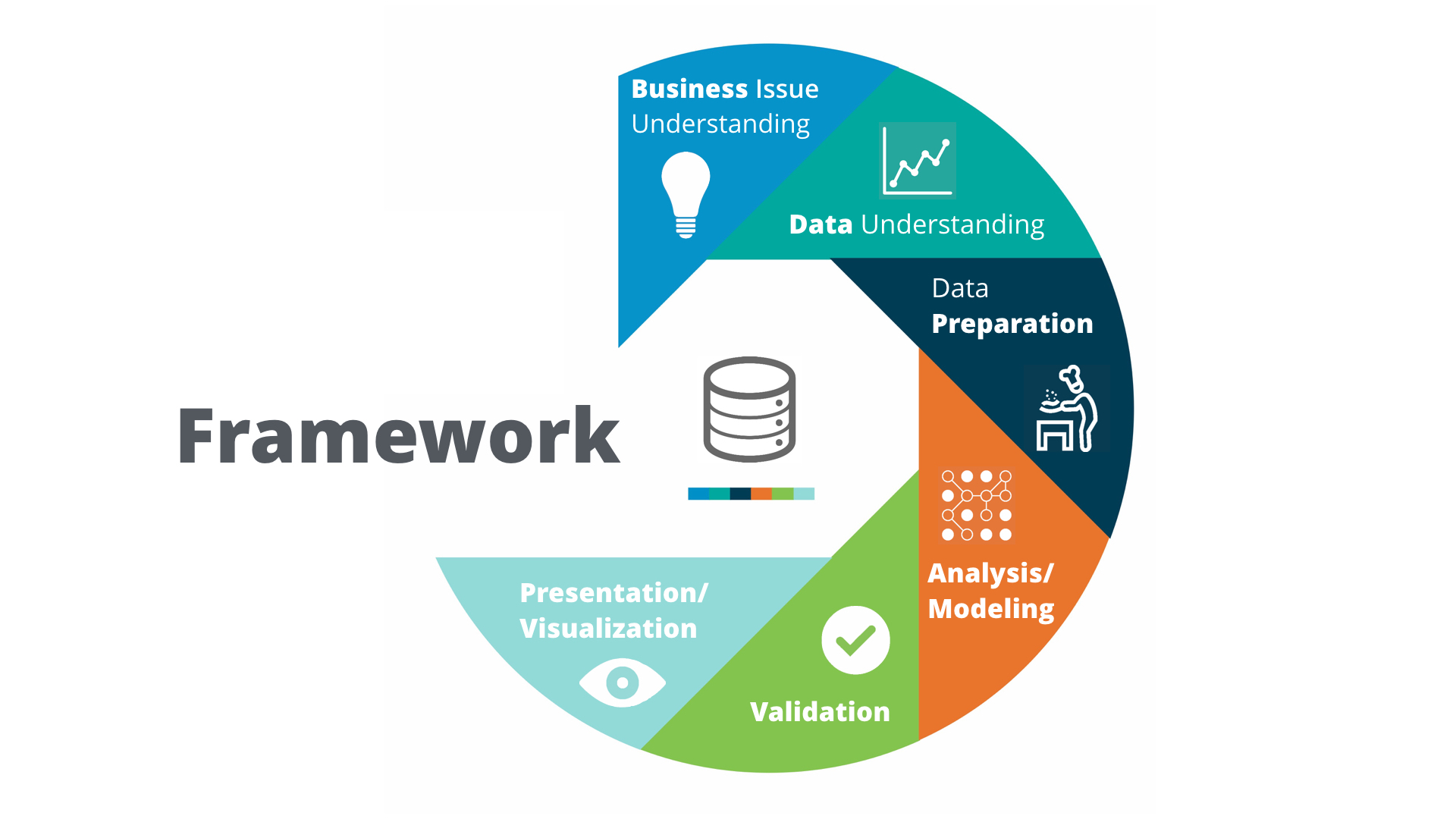
1.3 Analytical problem-solving framework

Problem-solving framework: Cross Industry Standard Process for Data Mining (CRISP-DM).
Smiley face
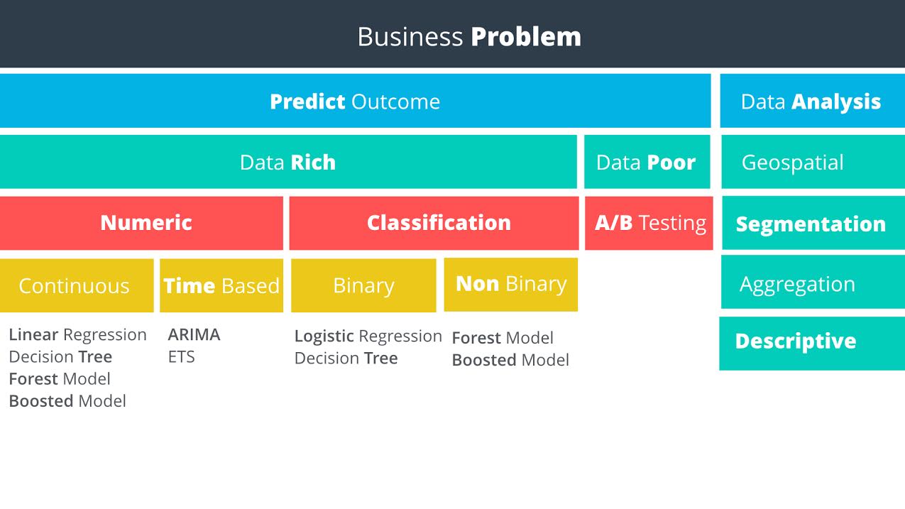
Predictive methodology map
Smiley face
Data rich vs data poor: Do you have data on what you want to predict?

1.5 Linear Regression

You can do single or multiple variable linear regression in Excel.
For categorical variables, it doesn’t make sense to assign value 1, 2, 3. Instead, it is better to use dummy variables, also called one hot encoding. Alteryx can do such things, but sadly, it has the only windows version. Alternatively, Weka is open source and has a mac version. Sadly again, it is ugly and can not even parse csv correctly.

1.5.21 interpreting linear regression results

P Value

The p-value is the probability that observed results (the coefficient estimate) occurred by chance, and that there is no actual relationship between the predictor and the target variable. In other words, the p-value is the probability that the coefficient is zero. The lower the p-value the higher the probability that a relationship exists between the predictor and the target variable. If the p-value is high, we should not rely on the coefficient estimate. When a predictor variable has a p-value below 0.05, the relationship between it and the target variable is considered to be statistically significant.
Statistical Significance - “Statistical significance is a result that is not likely to occur randomly, but rather is likely to be attributable to a specific cause.”
Note that p-values can be the ones for the coefficients of a linear model (sadly not provided by sklearn.linear_model.LinearRegression) or the one computed by a significance test from sklearn.feature_extraction

R-Squared

In our example, the R-squared value is 0.9651, and the adjusted R-squared value is 0.9558. Therefore, we’ve been able to improve the model with the addition of the category. In a real life problem, we might run the model with different predictor variables, or see if we had additional information to add to the model.
Remember, R-squared ranges from 0 to 1 and represents the amount of variation in the target variable explained by the variation in the predictor variables. The higher the r-squared, the higher the explanatory power of the model.

project 1: catalog campaign

key knowledge points:
  1. linear regression, including seaborn.regplot, seaborn.jointplot, sklearn.linear_model.Ridge, satsmodels.api.sm
  2. manipulate pandas DataFrame, including pandas.get_dummies, pandas.concat([], axis =1), pandas.drop(column, axis=1), df.dropna(axis=0,inplace=True)

2 data wrangling

data sources:

  1. computer file: MS Excel, Access,MapInfo, ArcGIS,SAS, SPSS,csv
  2. databases
  3. web-based sources

project 2.1: select a new store location

key pieces of knowledge:
  1. use the regular expression to search text.
  2. use bs4.BeautifulSoup(string,'html.parser').find(tag).text to extract data
  3. learn to make business decision

project 2.2: create report from database

SQL practice use software http://sqlitebrowser.org/ and chinook database.
notes:
  1. waste a lot of data on data visualization, especially how to control the size of axis, tickers, hue.
  2. use SQLite built-in function to parse daytime, such as strftime('%Y', string), strftime('%m', string). Or use date("now") to report time

3 data visualization

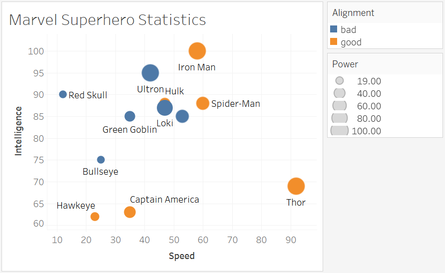
Tableau
Smiley face

Q1: How have movie genres changed over time?

This is a countplot by year and hue by genres.
I tried to do it in seaborn/matplotlib first, but surrendered to Tableau due to following reasons:
  1. genres are usually not single type, you have to split the string. Tableau is one click, Python do it by df['genres']= df['genres'].apply(lambda s: str(s).split("|")[0])
  2. countplot is actually an aggregation function + barplot. But 20 genres will make the barplot pretty ugly. So it is better to have line plot, which is easily done in Tableau. In python, a line of code sns.countplot(x = "release_year", hue = "genres", data = df[df["release_year"]>2000]) doesn’t give what you want. If you stick to python, then gb = df[df["release_year"]>2000].groupby(["release_year", "genres"]).count(), but groupby plot is not polished module. You get much more to do than necessity.
  3. python plot must decide which group of data to show. But you never know which one to show until you plot. In Tableau, just plot and use a filter to show the most important information,
Operation on Tableau:
  1. In data source, split the “Genre” which automatically takes first two.
  2. In Sheet,drag x value to “Columns”, y value to “Rows”, label value to “Marks” or “Filters”. The default setting for Measures type is an aggregation called SUM. That’s why when you drag two sets of numerical data, you don’t see scatter plot but a single one point. To avoid that, set it to Demesion.
  3. Aggregation is over all the records. To put aggregation on condition, SQL use on a = b group by c. Tableau does it by dragging data to Marks, the default granularity is details, which is just a subtle grid.
  • Question 2: How do the attributes differ between Universal Pictures and Paramount Pictures?
  • Question 3: How have movies based on novels performed relative to movies not based on novels? CONTAINS([Keywords], "novel")

5 classification models

The project is a binary classification. Dataset has shape (500,20). Most of the features are categorical.
Workflow:
  1. Examine each feature by seaborn.countplot() or seaborn.boxplot()
  2. drop features of bad quality: pd.drop(feature_list, axis=1, inplace = True)
  3. fillna with median value: data["Age-years"].fillna(median_age, inplace=True) median_age is preserved for latter unseen data
  4. make two variable lists: measures and dimensions
  5. dummies = pd.get_dummies(data[dimensions])
  6. a more secure way is to use from sklearn.preprocessing import OneHotEncoder because the encoder can remember the correct order and number in case unseen data has fewer classes.
  7. scale the numerical data by from sklearn.preprocessing import MinMaxScaler
  8. stack them together: features = np.hstack((hot, dummies.values,m))
  9. dummy target: target = pd.get_dummies(data["Credit-Application-Result"])['Creditworthy']
  10. time for machine learning:
from sklearn.model_selection import train_test_split
X_train, X_test, y_train, y_test = train_test_split(features, target, test_size = 0.3, random_state = 0)
from sklearn.tree import DecisionTreeClassifier
model = DecisionTreeClassifier()
model.fit(X_train, y_train)

from sklearn.metrics import accuracy_score
y_predict = model.predict(X_test)
score = accuracy_score(y_test, y_predict)
print("score: ", score) 

from sklearn.ensemble import RandomForestClassifier
from sklearn.svm import SVC
​