Deep Learning ND 3b, transfer learning,seq2seq

Recap:

https://jychstar.blogspot.com/2017/02/dlnd-0-intro-to-neural-network.html

https://jychstar.blogspot.com/2017/03/deep-learning-nd-2-sentiment-analysis.html

https://jychstar.blogspot.com/2017/03/deep-learning-nd-3-rnn-nlp.html

---

Project: Translation Project

14 Transfer learning

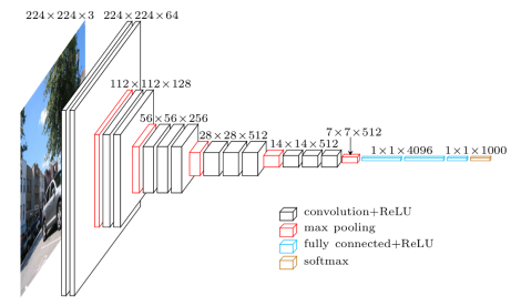
In this lesson, you’ll be using one of these pretrained networks, VGGNet, to classify images of flowers.

VGG (Visual Geometry Group), is an Oxford team led by Andrew Zisserman and Andrea Vedaldi. In VGGNet, only 3x3 convolution and 2x2 pooling are used throughout the whole network. It is quite famous because not only it works well, but the Oxford team have made the structure and the weights of the trained network freely available online. The Caffe weights are directly downloadable on the project’s web page; there are converted versions for other frameworks available around if you google them. One drawback of VGGNet is that this network is usually big. It contains around 160M parameters. Most of the parameters are consumed in the fc layers.

setup

git clone https://github.com/udacity/deep-learning.git
20170401
cd 20170401/transfer-learning
git clone https://github.com/machrisaa/tensorflow-vgg.git tensorflow_vgg
source activate py3
pip install tqdm
conda install scikit-image

“Transfer_Learning.ipynb” relies on tensorflow_vgg. Running the first code cell will download the parameter file (vgg16.npy, 553MB, ) from aws to the tensorflow_vgg folder.

This notebook is converted from the TensorFlow inception tutorial and shared the same dataset (flow_photos.tar.gz, 229MB). There are five classes: daisy (634 jpg files), dandelion (899), roses(642), sunflowers(700), tulips (800). A total of 3670 instances.

The complete VGGNet is 5 conv layers + 2 dense layers. Here, we only use the output of first 5 conv layers as a feature extractor. the input images have shape (244,244,3). vgg16.Vgg16().relu6 acts as a superpower image preprocessing machine that crush each image into fundamental pieces that are “really” ready for efficient classification. What exactly are these fundamental pieces? Maybe dots, lines, shapes, etc, we are not sure yet.

Supress warning by import warnings
warnings.filterwarnings("ignore") After my 2013 macbook painstakingly spinning for 6785s, I get these exciting pieces named as “codes“(60 MB). Each image or code is a vector with 4096 dimensions.

Then use a simple neural network with a 256-node layer to build a classifier. Train it and store it. Then randomly pick a flower image and let the fortune teller do the magic!

There are several tricks in vgg16.py to expedite the model building. The pre-trained parameter from vgg16.npy is loaded into Vgg16().data_dict during the class initialization and reset to None after building. It is computational expensive because of the many layers and huge number of parameters.

The filter size is stored by the name of the target layer. Each layer actually has multiple filters.

15 Sequence to Sequence

Instructor: Jay Alammar

Sequence to Sequence, published in 2014 by https://arxiv.org/abs/1409.3215, is one of RNN architectures that maps many to many.

One of the authors, Quoc Le, gave a talk: https://github.com/ematvey/tensorflow-seq2seq-tutorials

Chatbot dataset: Cornel Movie Dialogs Corpus, 200 k conversations from 600 movie scripts.

Stanford tutorial for chatbot

sequence to sequence tutorial: https://github.com/ematvey/tensorflow-seq2seq-tutorials

16 Deep Q learning

use neural networks to replace the Q-table.

gym

Project: language translation

It’s all about getting familiar with the RNN architectures using Tensorflow. The codes are almost identical to Course 15: seq2seq.

​

A gentle guide to start Extended Kalman Filter project

updated on 2017-6-18

I am moving very fast in term 2 and just finished all the projects in 3 weeks. In retrospect, uWebSocketIO is very necessary because all the projects have data IO with the simulator. And it’s a lot of fun watching the animation when you get the codes right.

Note: The reviewer will use the original “CMakeLists.txt” to judge your code. Although I recommend Clion IDE to facilitate debugging, make another copy for submission and make sure the following command works:

mkdir build && cd build
cmake .. && make
./mpc   # run it

---

This first project is overwhelming for C++ beginners wading from the Python world, where a lot of low-level implementation details have been hidden by the Python interpreter. The reasons why we use C++ in the self-driving car are:

1. C++ is much faster in running. The codes are already compiled beforehand.
2. C++ is more reliable. C++ is statically typed so the machine knows exactly how much memory should be allocated for each variable. And C++ has full-fledged object-oriented support so it is much easier to handle a large project.
3. C++ is more closed to the hardware. It is the first language for “Internet of things” devices. A particular example is that the electrical engineering students write C++ codes in mbed for ARM Cortex chip/microcontroller.

Now we get our mind in C++. For this EKF project, the major goal is to implement Kalman Matrix (using Eigen library). On 2017.5.3, Udacity introduced the simulator, which makes the result visually appealing, but may frustrate beginners due to the complicated setup of the uWebSocketIO.

In this blog, I will guide you through the basics by 3 steps. You can jump into step 3 to see how uWS is setup for Mac.

I use Macbook Pro OS X El Capitan (10.11.6). My C++ IDE is Clion (1 year free for a student). I recommend use Clion because each project folder is very clean: your source codes, a “CMakeLists.txt” and a “cmake-build-debug”folder (where you put the input.txt). I use CMake 3.7.2 and C++ 11.

You may need to spend a little time to understand how “CMakeLists.txt” works. Udacity provides such file for each project for term 2. If you use Clion, you only need to make a little changes and everything works like a charm.

1. practice Kalman Matrices locally

Practice locally to clear any blindspot.

Lesson 5.6 (Kalman Matrices 1D) is a good starting point. Learn how to use Eigen libraries and how matrix/vector works. There are 2 ways to include Eigen libraries depending on where you store them. Details see my note.

Lesson 5.12 (laser measurement 2D) is a mini-version of the EKF project. This is the best place to get familiar with the algorithm flow and how to link different source file together. My learning notes are here.

2. EKF without uWS

Download starter code from Udacity.

Create a copy. Compare two “main.cpp” files from lesson 5.12 and the starter code, delete everything about uWS. It will be easy if you already run 5.12 codes locally. There’s no trick in my “CMakeLists.txt” :

cmake_minimum_required(VERSION 3.7)
project(kf_p1) # kf_p1 is a project name I choose
set(CMAKE_CXX_STANDARD 11)
include_directories(/usr/local/Cellar/eigen/3.3.3/include/eigen3/)
add_executable(kf_p1 main.cpp kalman_filter.cpp FusionEKF.cpp tools.cpp)

Now you’re ready to dive into EKF project. Without the distraction of uWS, you can actually code and debug much more efficiently.

For example, you will encounter Assertion failed: (aLhs.rows() == aRhs.rows() && aLhs.cols() == aRhs.cols()), function CwiseBinaryOp,.... In other words, the dimensions of two related matrices are not aligned. The bad thing is that the compiler doesn’t tell you where the error happens. So you have to set some break points or use cout here and there to localize the error. You can do it more efficiently with a direct ifstream than json stream via uWS.

3. use uWebSocketIO

My workable “CMakeList.txt” looks like this:

cmake_minimum_required(VERSION 3.7)
project(kf_p1)
set(CMAKE_CXX_STANDARD 11)
include_directories(/usr/local/Cellar/eigen/3.3.3/include/eigen3/)
include_directories(/usr/local/include)
   link_directories(/usr/local/lib)
include_directories(/usr/local/Cellar/openssl/1.0.2k/include)
   link_directories(/usr/local/Cellar/openssl/1.0.2k/lib)
include_directories(/usr/local/Cellar/libuv/1.11.0/include)
   link_directories(/usr/local/Cellar/libuv/1.11.0/lib)
include_directories(/usr/local/Cellar/zlib/1.2.11/include)
   link_directories(/usr/local/Cellar/zlib/1.2.11/lib)
add_executable(kf_p1 main.cpp kalman_filter.cpp FusionEKF.cpp tools.cpp)
target_link_libraries(kf_p1 z ssl uv uWS)

Ideally, every include files should be in /usr/local/include and every lib files should be in /usr/local/lib. But brew install organize things differently and put them in /usr/local/Cellar/ by name and version.

To walk you through the setup, I will divide it into 2 steps.

1. install dependencies

The tricky thing is that uWS is built on 3 libraries (ssl, zlib, libuv). These 3 libraries can be easily installed by brew install openssl zlib libuv.

As you see in the “CMakeList.txt”, these 3 libraries all have a folder called “lib”. But uWS doesn’t have such thing because it is built on others. There may be also some environment dependencies so you will have to build it yourself in step 2.

For a similar reason, there is no brew install for uWs. You have to download it directly from its official github. However, the started code seems not compatible with the latest version 0.14 and will cause “onMessage” issue. So it is recommended to use version 0.13.

2. make uWS library

Udacity has provided a walk-through video and install-mac.sh file to do this. I am trying to fill the knowledge gap from my experience:

brew install openssl libuv cmake
git clone https://github.com/uWebSockets/uWebSockets 
cd uWebSockets
git checkout e94b6e1  # all files restored to v0.13
patch CMakeLists.txt < ../cmakepatch.txt  # revise "CMakeLists.txt" from "cmakepath.txt" in upper level folder
mkdir build  # create a new folder
export PKG_CONFIG_PATH=/usr/local/Cellar/openssl/1.0.2k/lib/pkgconfig # modify yours, check by "brew list openssl"
cd build
cmake ..   # produce a "Makefile" and a file folder
make    # use "Makefile" to compile sources into library
sudo make install # copy files to "/usr/local/..."
cd ..
cd ..
sudo rm -r uWebSockets

Several confusing things in the above:

1. “patch” command. “cmakepatch.txt” is provided by Udacity, and “CMakelists.txt” is provided by uWS. So make sure these 2 files are in the right place. Tricky thing is the latest UWebSockets only provides Makefile but no CMakelist.txt
2. What “cmakepatch.txt” does is to add command that will install libuWS.dylib to /usr/local/lib and copy a batch of .h files to /usr/local/include
3. I never get through cmake .. and make by following Udacity’s guide. I always get errors related to “openssl” and can’t figure out why. Thanks to Ian Zhang for providing the Makefile. It is based on the latest official uWS Makefile and adds one more line:”CPP_EXPERIMENTAL := -DUSE_MICRO_UV”. I use this file then everything works like a charm!
4. The last command is to remove the whole “uWebSockets” because it is not needed anymore. All the useful things have been copied to /usr/local/…

Final words

Despite I spend almost 2 days dealing with various tricky errors, it is worth the effort to get installed. I hope this guide can help you save some time and dive into the essentials.

​

Self-driving Car ND B1, Kalman Filter

Techniques for estimating the state of a system:

1. Kalman filter, for continuous state and unimodal distribution
2. Moute Carlo localization, for discrete state

Kalman Filter represents our distributions by Gaussians and iterates on 2 main cycles:

1. measurement update, Bayes rule
2. motion update(prediction), convolution, total probability

Distribution is described by a Guassian function:

1 measurement update

The new information will always decrease your covariance, meaning more certainty. Think about it this way: at , so the smaller sigma, the larger probability you have.

2 motion update

position is observable, speed is hidden and can be inferred from the location.

3 Kalman Matrices 1D

This is interesting. similar to the matrix representation of Quantum physics, we have matrix representation of Kalman filter. For convenience, location and velocity is wrapped together as x, the corresponding uncertainty is represented as P.

def kalman_filter(x, P):
    for n in range(len(measurements)):
        # measurement update
        Z = matrix([[measurements[n]]])
        y = Z-(H *x)  # error
        S = H * P * H.transpose() + R
        K = P * H.transpose() * S.inverse()  # Kalman gain
        x = x + (K*y)
        P = (I- (K*H)) *P
        # motion update
        x = (F*x) + u
        P = F*P * F.transpose()
    return x,P
measurements = [1, 2, 3]
x = matrix([[0.], [0.]]) # initial state (location and velocity)
P = matrix([[1000., 0.], [0., 1000.]]) # initial uncertainty
u = matrix([[0.], [0.]]) # external motion
F = matrix([[1., 1.], [0, 1.]]) # next state function
H = matrix([[1., 0.]]) # measurement function
R = matrix([[1.]]) # measurement uncertainty
I = matrix([[1., 0.], [0., 1.]]) # identity matrix
print kalman_filter(x, P)

In each iteration, we first have measurement update and then motion update. The key element in both updates is a very simple transfer matrix F=[[1,1],[0,1]]. For measurement update, because we can only directly measure location, so we extract the location from the state x by an even simpler matrix H =[1,0]. By comparing the old location and new measured location, we get error y. Combine with measurement uncertainty, we get a middle variable S and then Kalman gain K. Now we are ready to update the measurement state.

6 Kalman Matrices 1D by C++

#include <iostream>
#include <Eigen/Dense>
#include <vector>
using namespace std;
using namespace Eigen;
//Kalman Filter variables
VectorXd x,u;    // object state, external motion
MatrixXd P;    // object covariance matrix
MatrixXd F; // state transition matrix: 1, 1, 0, 1;
MatrixXd H, R;    // measurement matrix and covariance
MatrixXd I; // Identity matrix: 1,0,0,1
MatrixXd Q;    // process covariance matrix(noise):0,0,0,0

void filter(VectorXd &x, MatrixXd &P) {
    for (int n = 0; n < measurements.size(); ++n) {
        VectorXd z = measurements[n];
        VectorXd y = z- (H * x);
        VectorXd S = H * P* H.transpose() + R;
        VectorXd K = P * H.transpose() * S.inverse();
        // state update
          x = x + K * y;
        P = (I- K*H) * P;
          // motion update
        x = F *x +u;
        P = F*P* F.transpose()+Q;
    }
}

12 laser measurment 2D

The assignment is to implement Tracking::ProcessMeasurement(), which is only a very small part of the whole story. From bird’s eye view, there are several steps:

1. main.cpp first parse the input file and get the corresponding information into vector<MeasurementPackage>. Each “MeasurementPackage” includes long timestamp_, sensor_type_ and VectorXd raw_measurements_.
2. create a Tracking instance, in which the constructor initialize all the 6 parameters of KalmanFilter instance, as well as noise, initialized status and timestamp.
3. use the Tracking instance to process the “MeasurementPackage” by calling ProcessMeasurement(). The first measurement is used to initialize state and timestamp, others are used to modify transfer matrix F and process covariance Q.
4. call KalmanFilter::Predict()
5. call KalmanFilter::Update()

Note that class Kaman_filter and Tracking have been written in separate .h file and .cpp file. So the linking statement add_executable(kf main.cpp kalman_filter.cpp tracking.cpp)must be added into CMakeLIsts.txt.

Now it’s ready to get to the meat:

// Process a single measurement
void Tracking::ProcessMeasurement(const MeasurementPackage &measurement_pack) {
    if (!is_initialized_) {
        kf_.x_ << measurement_pack.raw_measurements_[0], measurement_pack.raw_measurements_[1], 0, 0;
        previous_timestamp_ = measurement_pack.timestamp_;
        is_initialized_ = true;
        return;
    }
    float dt = (measurement_pack.timestamp_ - previous_timestamp_) * 1e-6;    //dt - expressed in seconds
    previous_timestamp_ = measurement_pack.timestamp_;
    float dt_2 = dt *dt;
    float dt_3 = dt_2 *dt;
    float dt_4 = dt_3 *dt;
    kf_.F_(0, 2) = dt;
    kf_.F_(1, 3) = dt;
    kf_.Q_ = MatrixXd(4, 4);
    kf_.Q_ <<  dt_4/4*noise_ax, 0, dt_3/2*noise_ax, 0,
            0, dt_4/4*noise_ay, 0, dt_3/2*noise_ay,
            dt_3/2*noise_ax, 0, dt_2*noise_ax, 0,
            0, dt_3/2*noise_ay, 0, dt_2*noise_ay;
    //predict
    kf_.Predict();
    //measurement update
    kf_.Update(measurement_pack.raw_measurements_);
    std::cout << "x_= " << kf_.x_ << std::endl;
    std::cout << "P_= " << kf_.P_ << std::endl;
}

18 Radar and the polar coordinates

Radar sees a different world. It measures .

Extended Kalman Filter (EKF) uses a linear approximation of h(x), which is the first order approximation of Taylor expansion.

Because the original spaces have 4 variables: x, y, vx,vy. We will use a Jacobian matrix to represent the partial derivatives.

MatrixXd CalculateJacobian(const VectorXd& x_state) {
    MatrixXd Hj(3,4); // set size
    float px = x_state(0), py = x_state(1);
    float vx = x_state(2), vy = x_state(3);
    float c1 = px*px+py*py;
    float c2 = sqrt(c1);
    float c3 = (c1*c2);
    //check division by zero
    if(fabs(c1) < 0.0001){ // c-styple abs only for int
        cout << "Error - Division by Zero" << endl;
        return Hj;
    }
    //compute the Jacobian matrix
    Hj << (px/c2), (py/c2), 0, 0,
          -(py/c1), (px/c1), 0, 0,
          py*(vx*py - vy*px)/c3, px*(px*vy - py*vx)/c3, px/c2, py/c2;
    return Hj;
}

22 Calculate Root Mean Square Error

VectorXd CalculateRMSE(const vector<VectorXd> &estimations,
        const vector<VectorXd> &ground_truth){
    VectorXd rmse(4) = VectorXd::Zero(); //initialize
    if(estimations.size() != ground_truth.size()
            || estimations.size() == 0){
        cout << "Invalid data" << endl;
        return rmse;
    }
    //accumulate squared residuals
      VectroXd residual(4);
    for(unsigned int i=0; i < estimations.size(); ++i){
        residual = estimations[i] - ground_truth[i];
        rmse += residual.array()*residual.array();
    }
    rmse = rmse/estimations.size(); //mean
    rmse = rmse.array().sqrt();  // square root
    return rmse;
}

​