Recap:
Lesson 10-12, project 3:behavioral cloning, due on Apr. 17.
10: Keras
deep learning Frameworks
Andrew Gray, self-driving car engineering at OTTO (Uber)
Behavioral cloning, because the network clone human driving behavior. Sometimes it’s called end to end learning, because network only learns to predict the correct steering wheel angle and speed using only the inputs from the sensors.
Currently two approaches are used at OTTO:
- Traditional robotics approach, which requires a lot of detailed knowledge about sensors, controls, and planning.
- Deep learning approach, we simply feed all the information we have into the network, and then we let the network figure out on its own what’s important. Also there is a feedback loop and in turn it can teach us how to drive even better.
Both approaches are important. Traditional approach gives you a intuitive way to understand how it works and gain insights, while deep learning as a magic black box can maximize the performance.
Neural Networks in Keras
Example 1: a simple network with 3 densed layers for input images of 32x32.
import tensorflow as tf
tf.python.control_flow_ops = tf
from keras.models import Sequential
from keras.layers.core import Dense, Activation, Flatten, Dropout
from keras.layers.convolutional import Convolution2D
from keras.layers.pooling import MaxPooling2D
# preprocess data
X_normalized = np.array(X_train / 255.0 - 0.5 )
X_normalized_test = np.array(X_test / 255.0 - 0.5 )
from sklearn.preprocessing import LabelBinarizer
label_binarizer = LabelBinarizer()
y_one_hot = label_binarizer.fit_transform(y_train)
y_one_hot_test = label_binarizer.fit_transform(y_test)

# build a neural network with 2 dense layers
n_class = 10
model = Sequential()
model.add(Flatten(input_shape=(32, 32, 3)))
model.add(Dense(128))
model.add(Activation('relu'))
model.add(Dense(n_class))
model.add(Activation('softmax'))
model.compile('adam', 'categorical_crossentropy', ['accuracy'])
# train
history = model.fit(X_normalized, y_one_hot, nb_epoch=10, validation_split=0.2)

# test
metrics = model.evaluate(X_normalized_test, y_one_hot_test)
print()
for metric_i in range(len(model.metrics_names)): # ['loss', 'acc']
    metric_name = model.metrics_names[metric_i]
    metric_value = metrics[metric_i]
    print('{}: {}'.format(metric_name, metric_value))
Example 2: a neural network with 1 convolutional layer, maxpooling, dropout
model = Sequential()
model.add(Convolution2D(32, 3, 3, input_shape=(32, 32, 3)))
model.add(MaxPooling2D((2, 2)))
model.add(Dropout(0.5))
model.add(Activation('relu'))
model.add(Flatten())
model.add(Dense(128))
model.add(Activation('relu'))
model.add(Dense(5))
model.add(Activation('softmax'))
11 Transfer Learning
Bryan Catanzaro, an author of NVIDIA cuDNN, worked on Baidu speech recognition
4 types of transfer, depending on dataset size and similarity.

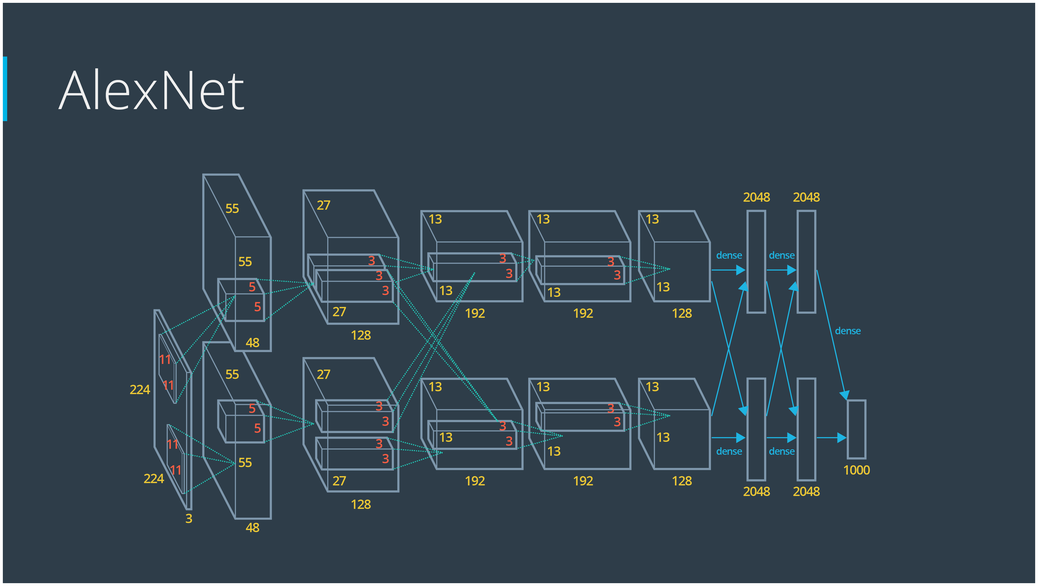
Alexnet
AlexNet, designed by Alex Krizhevsky, is the winner of 2012 ImageNet competition. It makes deep learning regain popularity overnight.
- 5 convolutional layers + 3 dense layers
- Use the best GPU to train for a week
- ReLu, dropout
- error rate drop from 26% to 15%
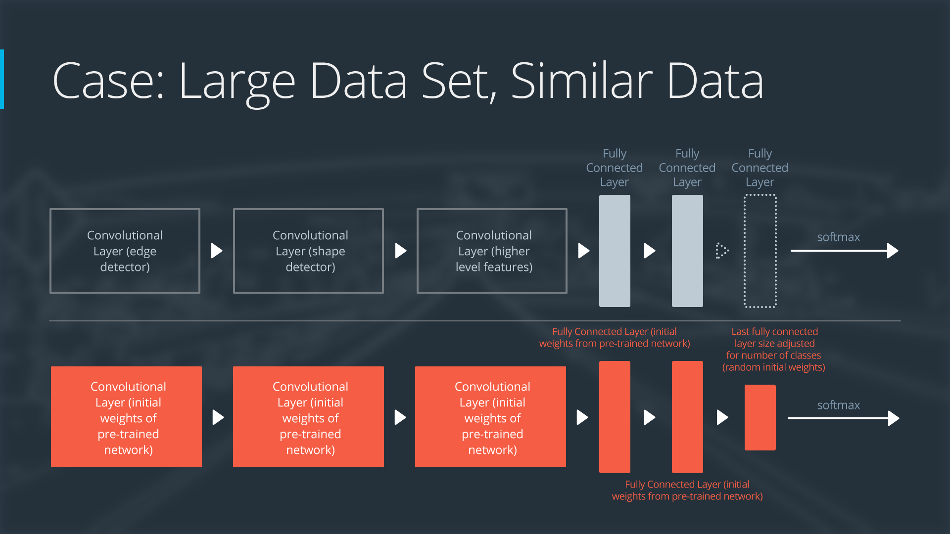
2 popular methods to apply transfer learning:
- Feature extraction: replace the final layer, freeze all the previous layer
- Fine tuning: all layers are retrained end-to-end
use original Alexnet: no retrain
Exercise codes at https://github.com/udacity/CarND-Alexnet-Feature-Extraction , which is adapted from https://github.com/ethereon/caffe-tensorflow The original codes was written in caffe framework.
The detailed architecture of Alexnet is:
- conv1, lrn1, maxpool1
- conv2, lrn2, maxpool2
- conv3
- conv4
- conv5, maxpool5
- fc6 (4096)
- fc7 (4096)
- fc8 (1000)
The pre-trained parameters for kernels, weights and bias are stored in
bvlc-alexnet.npy(240 MB).
Note that the input image has shape of (227,227,3) and output is the probabilities for 1000 classes. Decoding for these classes is done by a dictionary stored in
caffe_classes.class_namesfeature extraction + retrain
Obviously, the drawback of this complete alexnet model is its limitation on these 1000 classes. It is no surprise that a stop sign is recognized as digital watch/clock.
Alternatively, we replace the last layer with a dimention matched to the traffic sign classes:
sign_names = pd.read_csv('signnames.csv')
nb_classes = 43
x = tf.placeholder(tf.float32, (None, 32, 32, 3))
resized = tf.image.resize_images(x, (227, 227)) # resize
fc7 = AlexNet(resized, feature_extract=True)
shape = (fc7.get_shape().as_list()[-1], nb_classes) # 4096
fc8W = tf.Variable(tf.truncated_normal(shape, stddev=1e-2))
fc8b = tf.Variable(tf.zeros(nb_classes))
logits = tf.nn.xw_plus_b(fc7, fc8W, fc8b)
probs = tf.nn.softmax(logits)
If we feed 26.27 k instances into training, a GTX 970 will take 1 minute, but my poor 2013 MacBook take 200 minutes.
GoogLeNet, VGG
Andrew Gray
deep learning is a hands-on empirical field. The more experients our engineers and researchers try, the more ideas we generate. Some work and some doesn’t work. The practice is ahead of theory in many cases. So it’s important not to get attached to theories about different network architectures, exactly what layer followers another. You need to bias towards action, experiment to answer your questions rather than just thinking deep thoughts.These experiments make us real scientists.
The competition is fierce:

ImageNet winner in 2014 is googLeNet (inception v1) 6.7%, and VGG 7.3%,


practice: simple CNN vs pretrained model
practice codes at https://github.com/udacity/CarND-Transfer-Learning-Lab
Benchmark:
cifar10 dataset, 50 k/10k train/test set, 1cnn+2 dense layer lead to 0.664 accuracy in 10 epoch.
With keras, the code implementation is much easier:
import tensorflow as tf
tf.python.control_flow_ops = tf
from keras.models import Sequential
from keras.layers.core import Dense, Activation, Flatten, Dropout
from keras.layers.convolutional import Convolution2D
from keras.layers.pooling import MaxPooling2D
# preprocess data
X_normalized = np.array(X_train / 255.0 - 0.5 )
X_normalized_test = np.array(X_test / 255.0 - 0.5 )
from sklearn.preprocessing import LabelBinarizer
label_binarizer = LabelBinarizer()
y_one_hot = label_binarizer.fit_transform(y_train)
y_one_hot_test = label_binarizer.fit_transform(y_test)

# build a neural network with 2 dense layers
n_class = 10
model = Sequential()
model.add(Convolution2D(32, 3, 3, input_shape=(32, 32, 3)))
model.add(MaxPooling2D((2, 2)))
model.add(Dropout(0.5))
model.add(Activation('relu'))
model.add(Flatten())
model.add(Dense(128))
model.add(Activation('relu'))
model.add(Dense(n_class))
model.add(Activation('softmax'))
model.compile('adam', 'categorical_crossentropy', ['accuracy'])
# train
history = model.fit(X_normalized, y_one_hot, nb_epoch=10, validation_split=0.2)

# test
metrics = model.evaluate(X_normalized_test, y_one_hot_test)
print()
for metric_i in range(len(model.metrics_names)): # ['loss', 'acc']
    metric_name = model.metrics_names[metric_i]
    metric_value = metrics[metric_i]
    print('{}: {}'.format(metric_name, metric_value))
Feature extraction:
bottle-neck features (preprocessed by the pre-trained models) such as vgg, inception and resnet use 1k/10k train/test set, 1 dense layer as the final output, only get ~0.70 accuracy in 50 epoch. 2 dense layer as the final output will get 0.756 accuracy. So these superpower technologies kind of overkill/overtrain.
Because the pre-trained models have done the dirty job that converts the images into cnn outputs, the implementation only takes care of the last part.
import pickle
import tensorflow as tf
import numpy as np
# load data
training_file = "vgg_cifar10_100_bottleneck_features_train.p"
validation_file = "vgg_cifar10_bottleneck_features_validation.p"
# load bottleneck data
with open(training_file, 'rb') as f:
    train_data = pickle.load(f)
with open(validation_file, 'rb') as f:
    validation_data = pickle.load(f)
X_train, y_train= train_data['features'], train_data['labels']
X_val, y_val = validation_data['features'], validation_data['labels']
nb_classes = len(np.unique(y_train))
epochs = 50
batch_size = 256
# define model
from keras.models import Sequential
from keras.layers import Flatten, Dense, Activation
input_shape = X_train.shape[1:] # vgg (1,1,512), inception (1,1,2048), Resnet (1,1,2048)
model = Sequential()
model.add(Flatten(input_shape=input_shape))
model.add(Dense(128))
model.add(Activation('relu'))
model.add(Dense(nb_classes))
model.add(Activation('softmax'))
model.compile(optimizer='adam', loss='sparse_categorical_crossentropy', metrics=['accuracy'])
# train model
model.fit(X_val, y_val, nb_epoch=epochs, batch_size=batch_size, validation_data=(X_train, y_train), shuffle=True)
To end this lab, let’s summarize when we should consider:
- Feature extraction (train only the top-level of the network, the rest of the network remains fixed)
- Finetuning (train the entire network end-to-end, start with pre-trained weights)
- Training from scratch (train the entire network end-to-end, start from random weights)
Finally, keep in mind that for a lot of problems you won’t need an architecture as complicated and powerful as VGG, Inception, or ResNet. These architectures were made for the task of classifying thousands of complex classes. A smaller network might be a better fit for a smaller problem, especially if you can comfortably train it on moderate hardware.
No comments:
Post a Comment
Note: Only a member of this blog may post a comment.