Self-driving Car ND A4, Advanced lane line, ending summary

Course 16, Project 4: Advanced Lane Finding

The following are my notes. Each section is labeled by the lesson number.

1 computer vision

Robotics can be broken down into a 3-step cycle:

1. sense or perceive the world
2. what to do based on the perception
3. perform an action to carry out that decision

Sebastian,

80% of the challenge of building a self-driving car is perception.

Use camera because it has better spatial resolution and much cheaper, although it lacks the 3D information that can ba captured by Lidar.

4 why correct image distortion?

1. apparent size
2. apparent shape
3. appearance change depending on the position
4. make object closer or farther than they actually are.

pinhole camera images are free from distortion, but lenses tend to introduce image distortion.

9 Finding corners

setup

sudo pip install matplotlib --upgrade

documentation: cv2.findChessboardCorners() and cv2.drawChessboardCorners().

image = cv2.imread(fname)  # bgr, (960, 1280, 3)
gray = cv2.cvtColor(image, cv2.COLOR_BGR2GRAY) #(960, 1280)
ret, corners = cv2.findChessboardCorners(gray, (nx, ny)) # bool, shape(48, 1, 2)
if ret == True:
    cv2.drawChessboardCorners(image, (nx, ny), corners, ret)
    plt.imshow(img)
    plt.show()

10 camera calibration

Course material: https://github.com/udacity/CarND-Camera-Calibration

The basic workflow:

1. take multiple pictures for the same image, e.g., chessboard, which serves as the ground truth. These ordered 3D points can be easily created by

   objp = np.zeros((6*8,3), np.float32)
   objp[:,:2] = np.mgrid[0:8, 0:6].T.reshape(-1,2)
   

2. For each image, find corners by cv2.findChessboardCorners(gray, (nx, ny)) and append to imgpoints.
3. use objpoints-imgpoints pairs, gray shape to extract calibrate parameters such as mtx (camera matrix, shape (3,3)) and dist (distortion coefficient, shape(1,5)).
4. undistort image and compare them side by side.

ret, mtx, dist, rvecs, tvecs = cv2.calibrateCamera (objpoints, imgpoints, gray.shape,None,None)
undistort = cv2.undistort(original, mtx, dist, None, mtx)

17 perspective transform

The goal is to get lane curvature

import cv2
from sklearn.externals import joblib
f= "calibration_wide/wide_dist_pickle.p"
mtx, dist = joblib.load(f)
img = cv2.imread('calibration_wide/GOPR0070.jpg')
nx, ny =8, 6  
undist = cv2.undistort(img, mtx, dist, None, mtx)
ret, corners = cv2.findChessboardCorners(undist[:,:,0], (8,6), None) 
if ret == True:
    cv2.drawChessboardCorners(img, (nx, ny), corners, ret)
    src = np.float32([corners[0], corners[nx-1], corners[-1], corners[-nx]]) # clockwise
    dst = np.float32([[0, 0],[1280, 0], [1280, 960],[0, 960]]) 
    M = cv2.getPerspectiveTransform(src, dst)
    top_down = cv2.warpPerspective(undist, M, (1280,960))

20 get gradience by sobel operator

Canny Edge detection algorithm is great that we can find all the edges and lines with the help of Hough space. To filter out the annoying undesirable edges, we narrow our focus on gradient along the x-direction. This is what the sobel operation comes in.

1. gradient of x: sobelx = cv2.Sobel(gray, cv2.CV_64F, 1, 0, ksize =3)
2. gradient magnitude: gradmag = np.sqrt(sobelx**2 + sobely**2)
3. direction of magnitude: np.arctan2(np.absolute(sobely), np.absolute(sobelx)) Direction alone is not particularly useful because there are directions everythere in every direction
4. combine.

# get the derivative in the x direction denoted by 1,0
sobelx = cv2.Sobel(gray, cv2.CV_64F, 1, 0, ksize = 3) 
sobely = cv2.Sobel(gray, cv2.CV_64F, 0, 1)
# normalize into (0,255)
abs_sobelx = np.absolute(sobelx)
scaled_sobel = np.uint8(255*abs_sobelx/np.max(abs_sobelx)) 
# select pixels based on the x gradient strength
sxbinary = np.zeros_like(scaled_sobel)
sxbinary[(scaled_sobel >= 20) & (scaled_sobel <= 100)] = 1 
# gradient magnitude
gradmag = np.sqrt(sobelx**2 + sobely**2)
gradmag = np.zeros_like(scaled_sobel)
gradmag[(gradmag >= 0) & (gradmag <= 200)] = 1 
# direction of the gradient
absgraddir = np.arctan2(np.absolute(sobely), np.absolute(sobelx))
dir_binary =  np.zeros_like(absgraddir)
dir_binary[(absgraddir >= 0)&(absgraddir <= np.pi)] = 1
# combine the selection threshold
combined = np.zeros_like(dir_binary)
combined[((gradx == 1) & (grady == 1)) | ((mag_binary == 1) & (dir_binary == 1))] = 1

26 color space

RGB issues: B channel does not detect yellow lane line. All channels vary under different levels of brightness.

wiki of HLS and HSV color spaces here.

(Hue, Saturation, Value) and (Hue, Lightness, Saturation) are very similar.

Hue, the range of (0,179), represents color independent of any change in brightness.

Lightness and Value represent different ways to measure the relative lightness or darkness of a color. For example, a dark red will have a similar hue but much lower value for lightness than a light red.

Saturation is a measurement of colorfulness: the brighter a single color, the higher saturation value; closer to white is lower saturation value.

H and S channels stay fairly consistently in shadow or excessive brightness. S seems to detect lane line pretty well, as well as the dark section of H channel.

28 color threshold

Red: (200,255)

S: (90,255)

H: (15,100)

After some experiments, S is better for yellow lines, R is better for white lines.

1. gradient x of lightness + raw value of saturation to create the binary image. threshold setting: (20,100), (170,255)

33 finding the lines

1. np.copy() RGB image, and by setting the low-value pixels to zero, only the high-value pixels are preserved
2. np.sum(img_cut[:,:,0], axis = 0) to get y intensity count over x-direction, such to estimate the lane line position by 2 peaks
3. use 9 windows to narrow down the position of lane lines. In each loop, define a window by center and margin, identify nonzeros pixels, which will be used for fitting parabolic equation, use np.mean() to get new centers for current windows
4. use np.concatenate() to merge points and use np.polyfit(y,x,2) to get coefficient of function x=f(y)
5. use np.linspace(min,max,num) to generate y points and use fitted coefficient to get the parabolic curves.
6. with initial fitting parameters at hand, search possible pixels in the neighborhood of fitting curves for subsequent images.
7. alternatively, use initial center points, np.convolve, and np.argmax to get the new centers and windows. But this approach doesn’t collect enough points to fit parabolic curves.

34 sliding window search: convolution

1. use np.sum and np.convolve to get the new centers for each window. This way is more mathematically and may be more dynamically robust.
2. b,g,r = cv2.split(img) and img = cv2.merge((b,g,r)) to deal with different color channels.
3. cv2.addWeighted() to add mask, this is equal to ax1+bx2

35 measure curvature

The radius of curvature (awesome tutorial here).

, A has unit of inverse length

def curverature(fit, y):
    A, B = fit[0], fit[1]
    return ((1+2*A*y+B)**2)**1.5/np.absolute(2*A)
# Define conversions in x and y from pixels space to meters
ym_per_pix = 30/720 # meters per pixel in y dimension
xm_per_pix = 3.7/700 # meters per pixel in x dimension

# Fit new polynomials to x,y in world space
left_fit_cr = np.polyfit(ploty*ym_per_pix, leftx*xm_per_pix, 2)
right_fit_cr = np.polyfit(ploty*ym_per_pix, rightx*xm_per_pix, 2)
# Calculate the new radii of curvature
left_curverad = ((1 + (2*left_fit_cr[0]*y_eval*ym_per_pix + left_fit_cr[1])**2)**1.5) / np.absolute(2*left_fit_cr[0])
right_curverad = ((1 + (2*right_fit_cr[0]*y_eval*ym_per_pix + right_fit_cr[1])**2)**1.5) / np.absolute(2*right_fit_cr[0])
#

36 project tips

the project repository

• camera calibration is a different setting: 9x6 chessboard. It is stored in “camera_cal” folder.
• expect the curvation to be around 1 km
• keep track of line base and curvatures from frame to frame.
• smooth out by average
• use cv2.warpPerspective(color_warp, Minv, image.shape[0:2]) to generate filled area that represent the found laneline and add to the original image

My implementation: https://github.com/jychstar/NanoDegreeProject

Produced video is uploaded to https://youtu.be/xZK199K9jwk

I want to highlight 3 points:

1. perspective transform needs some ground-truth facts to deal with the depth perception
2. know when to use sobel operation and color space. For this project, Red channel is enough for the “not challenged” video
3. know how to use a histogram to estimate the laneline base, use window search to collect qualified points, use initial fitting coefficient to quickly localize points for the subsequent images.

End of term 1 summary

First, in the 5 projects:

• 2 projects are about finding lanelines, either a straight line or curved lines. These projects are about computer vision.
• 2 projects are about identifying objects, either traffic signs or other vehicles. These projects are about deep learning.
• 1 projects are about end-to-end learning. This is still deep learning.

Second, this nanodegree helps me demystify how an autonomous car works. Although there are some tricky bugs that bother me a lot, I learn a lot.

Thank you, Udacity and Sebastian!

​

Self-driving Car ND A5, Vehicle detection

course 20, Project 5: Vehicle Detection and Tracking

Detailed implementation is in my github.

The following are my notes. Each section is labelled by the lesson number.

5 draw a blue box over the image

cv2.rectangle(image_to_draw_on, (x1, y1), (x2, y2), color=(0, 0, 255), thick=6)

(x1, y1) and (x2, y2) are the x and y coordinates of any two opposing corners of the bounding box you want to draw

6 feature intuition

features	characteristics
raw pixel intensity	color and shape
histogram of pixel intensity	color only
gradients of pixel intensity	shape only

9 template matching

compare a picture with an known image, the area that passes threshold is selected and its location is output.

result = cv2.matchTemplate(img, ref, cv2.TM_CCOEFF_NORMED)
min_val, max_val, min_loc, max_loc = cv2. minMaxLoc(result)  
height, weight, color = ref.shape
top_left = min_loc
bottom_right = (top_left[0] + w, top_left[1] + h)
bbox_list.append((top_left, bottom_right))

However, template matching is only useful for things that do not vary in their appearance much.

12 histogram of color

import matplotlib.image as mpimg
import numpy as np
image = mpimg.imread('cutout1.jpg') # RGB
rhist = np.histogram(image[:,:,0], bins=32, range=(0, 256))  # counts, edges: lengths are 32, 33
ghist = np.histogram(image[:,:,1], bins=32, range=(0, 256))
bhist = np.histogram(image[:,:,2], bins=32, range=(0, 256))
# Generating bin centers, one size for three
bin_edges = rhist[1]
bin_centers = (bin_edges[1:]  + bin_edges[:-1])/2
# Plot a figure with all three bar charts
plt.figure(figsize=(12,3))
plt.subplot(131)
plt.bar(bin_centers, rhist[0])
plt.xlim(0, 256)
plt.title('R Histogram')

15 explore color spaces

3d plot in rgb space and vhs space. code snippet:

https://gist.github.com/jychstar/0daa6ea1a8a759a279092042f396049b

16 spatial binning of color

cv2.resize(rgb_image, (32,32)).ravel()

reduce the size and flatten, nothing fancy.

20 histogram of orientation gradient (HOG)

The dataset for practice is vehicles_smallset and non-vehicles_smallset, each has about 1.2k jpeg files with size 64x64 and memory size of 5M in total.

skimage.feature.hog() is nice to calculate the hog of a gray image at one line of code.

There are several parameters to tune the hog:

1. orientations: number of directions you want to calculate.
2. pixels_per_cell: cell size over which each gradient histogram is computed.
3. cells_per_block: the local area over which the histogram counts in a given cell will be normalized.
4. visualise=True flag tells the function to output a visualization called hog_image, which shows a representation that shows the dominant gradient direction.
5. feature_vector=True flag is supposed to unroll the features, like ravel() But some bug cause it fail to unroll. So features has a shape of (7, 7, 2, 2, 9). Note that the length of gradient is always one less than orginal length.

By the way, the current version of skimage is 0.13. But my 0.12 version faisl to upgrade to this version.

from skimage.feature import hog
features, hog_image = hog(gray, orientations=9, pixels_per_cell=(8, 8), cells_per_block=(2, 2), visualise=True, feature_vector=False)

22 combine and normalize

rgb = mpimg.imread(path)  # (64, 64, 3)
spatial_features = cv2.resize(rgb, (32,32)).ravel() #(3072,)
rhist = np.histogram(rgb[:,:,0], bins=32, range=(0,256)
ghist = np.histogram(rgb[:,:,1], bins=32, range=(0,256)
bhist = np.histogram(rgb[:,:,2], bins=32, range=(0,256)
hist_features = np.concatenate((rhist[0], ghist[0], bhist[0]))  # (96,)
feature = np.concatenate((spatial_features, hist_features))  # (3168,)
scaler = sklearn.preprocessing.StandardScaler(copy=True, with_mean=True, with_std=True) # define standard scaler, mean 0
scaler.fit(X) # separate fit/transform to process unseen data
scaled_X = scaler.transform (X)

28 svc classifier by raw color

input feature is raw color + histogram of rgb channel, so input dimension is 2321x3169. Note that X is built by np.vstack, y is built by np.hstack

using sklearn.svm.LinearSVC() and train_test_split, it takes 0.6 s to train and get 0.98 test accuracy.

29 svc classifier by HOG

input feature is HOG of r channel, so input size: 2321x1764, takes 0.11 s, 0.975 accuracy.

if use HOG of rgb channels, input size: 2321x5292, takes 0.24s, 0.98 accuracy

32 sliding window

build a list of sliding windows. window size (128,128)

https://gist.github.com/jychstar/7eef27dbb3b7ac5e77a3f7e9724bd70f

34 search and classify

1. stack raw color, histogram of color, histogram of gradient as input features. so feature length = . So the HOG features are dominant.
2. train a classifier
3. crop the input image to a series of 64x64 images by sliding windows and resize it to the train image shape, do the same preprocessing and apply classifier
4. if true, save the window positions and draw on the image

35 subsample

some optimizations/tricks:

1. use YCrCb color space
2. use cells per step instead of overlap
3. crop lower half of the image,y=(400,656) and apply scale factor=1.5
4. directly slice from HOG data

37 multiple detection and false positive

1. create a heatmap initialized with 0,
2. the area covered by detected boxes adds value 1, multiple detection areas will have value more than 1
3. set threshold and reset small value area back to 0
4. labels,num = scipy.ndimage.measurements.label(heatmap) identify the objects by locations and numbers. Any non-zero values in input are counted as features and zero values are considered the background.
5. use labels to cut out each object and draw

​

Self-driving Car ND A3,, transfer learning, behavioral cloning

Recap:

https://jychstar.blogspot.com/2017/02/scnd-11-finding-lane.html

https://jychstar.blogspot.com/2017/04/self-driving-car-nd-a2-traffic-sign.html

---

Lesson 10-12, project 3:behavioral cloning, due on Apr. 17.

10: Keras

deep learning Frameworks

Andrew Gray, self-driving car engineering at OTTO (Uber)

Behavioral cloning, because the network clone human driving behavior. Sometimes it’s called end to end learning, because network only learns to predict the correct steering wheel angle and speed using only the inputs from the sensors.

Currently two approaches are used at OTTO:

1. Traditional robotics approach, which requires a lot of detailed knowledge about sensors, controls, and planning.
2. Deep learning approach, we simply feed all the information we have into the network, and then we let the network figure out on its own what’s important. Also there is a feedback loop and in turn it can teach us how to drive even better.

Both approaches are important. Traditional approach gives you a intuitive way to understand how it works and gain insights, while deep learning as a magic black box can maximize the performance.

Neural Networks in Keras

Example 1: a simple network with 3 densed layers for input images of 32x32.

import tensorflow as tf
tf.python.control_flow_ops = tf
from keras.models import Sequential
from keras.layers.core import Dense, Activation, Flatten, Dropout
from keras.layers.convolutional import Convolution2D
from keras.layers.pooling import MaxPooling2D
# preprocess data
X_normalized = np.array(X_train / 255.0 - 0.5 )
X_normalized_test = np.array(X_test / 255.0 - 0.5 )
from sklearn.preprocessing import LabelBinarizer
label_binarizer = LabelBinarizer()
y_one_hot = label_binarizer.fit_transform(y_train)
y_one_hot_test = label_binarizer.fit_transform(y_test)

# build a neural network with 2 dense layers
n_class = 10
model = Sequential()
model.add(Flatten(input_shape=(32, 32, 3)))
model.add(Dense(128))
model.add(Activation('relu'))
model.add(Dense(n_class))
model.add(Activation('softmax'))
model.compile('adam', 'categorical_crossentropy', ['accuracy'])
# train
history = model.fit(X_normalized, y_one_hot, nb_epoch=10, validation_split=0.2)

# test
metrics = model.evaluate(X_normalized_test, y_one_hot_test)
print()
for metric_i in range(len(model.metrics_names)): # ['loss', 'acc']
    metric_name = model.metrics_names[metric_i]
    metric_value = metrics[metric_i]
    print('{}: {}'.format(metric_name, metric_value))

Example 2: a neural network with 1 convolutional layer, maxpooling, dropout

model = Sequential()
model.add(Convolution2D(32, 3, 3, input_shape=(32, 32, 3)))
model.add(MaxPooling2D((2, 2)))
model.add(Dropout(0.5))
model.add(Activation('relu'))
model.add(Flatten())
model.add(Dense(128))
model.add(Activation('relu'))
model.add(Dense(5))
model.add(Activation('softmax'))

11 Transfer Learning

Bryan Catanzaro, an author of NVIDIA cuDNN, worked on Baidu speech recognition

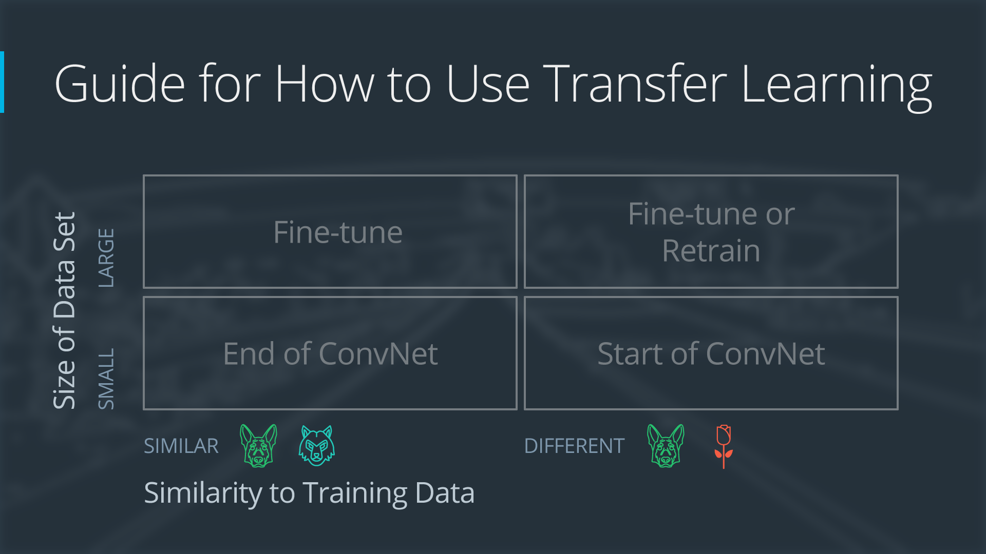
4 types of transfer, depending on dataset size and similarity.

Alexnet

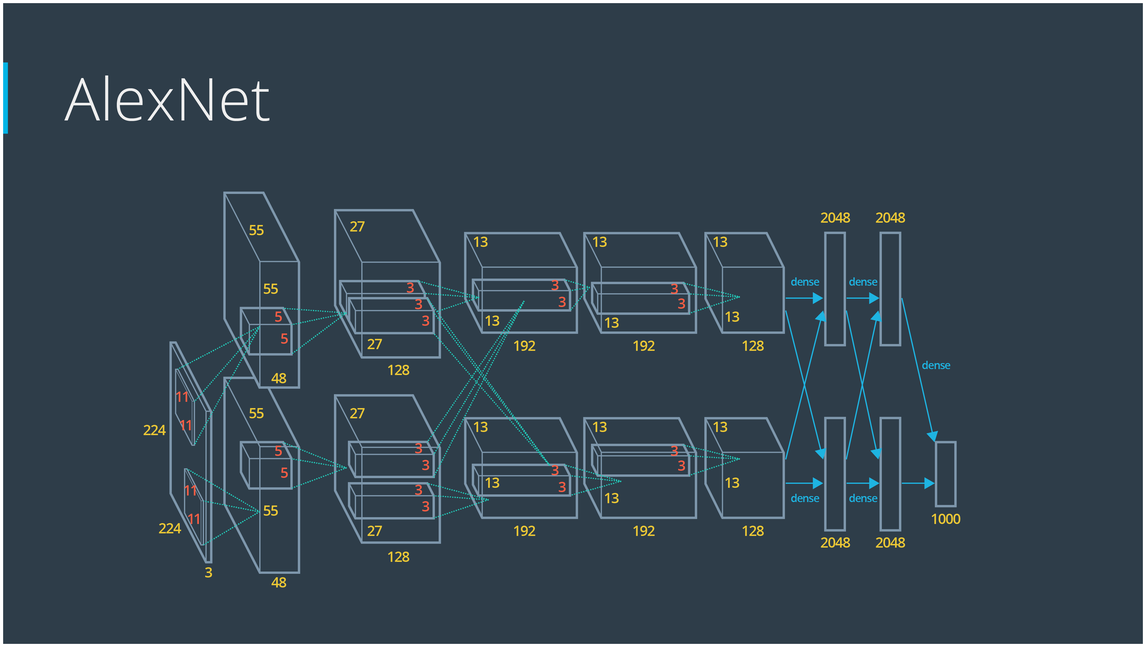
AlexNet, designed by Alex Krizhevsky, is the winner of 2012 ImageNet competition. It makes deep learning regain popularity overnight.

• 5 convolutional layers + 3 dense layers
• Use the best GPU to train for a week
• ReLu, dropout
• error rate drop from 26% to 15%

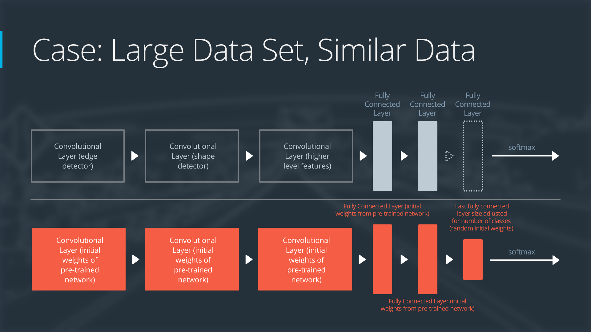
2 popular methods to apply transfer learning:

• Feature extraction: replace the final layer, freeze all the previous layer
• Fine tuning: all layers are retrained end-to-end

use original Alexnet: no retrain

Exercise codes at https://github.com/udacity/CarND-Alexnet-Feature-Extraction , which is adapted from https://github.com/ethereon/caffe-tensorflow The original codes was written in caffe framework.

The detailed architecture of Alexnet is:

1. conv1, lrn1, maxpool1
2. conv2, lrn2, maxpool2
3. conv3
4. conv4
5. conv5, maxpool5
6. fc6 (4096)
7. fc7 (4096)
8. fc8 (1000)

The pre-trained parameters for kernels, weights and bias are stored in bvlc-alexnet.npy(240 MB).

Note that the input image has shape of (227,227,3) and output is the probabilities for 1000 classes. Decoding for these classes is done by a dictionary stored in caffe_classes.class_names

feature extraction + retrain

Obviously, the drawback of this complete alexnet model is its limitation on these 1000 classes. It is no surprise that a stop sign is recognized as digital watch/clock.

Alternatively, we replace the last layer with a dimention matched to the traffic sign classes:

sign_names = pd.read_csv('signnames.csv')
nb_classes = 43
x = tf.placeholder(tf.float32, (None, 32, 32, 3))
resized = tf.image.resize_images(x, (227, 227)) # resize
fc7 = AlexNet(resized, feature_extract=True) 
shape = (fc7.get_shape().as_list()[-1], nb_classes) # 4096
fc8W = tf.Variable(tf.truncated_normal(shape, stddev=1e-2))
fc8b = tf.Variable(tf.zeros(nb_classes))
logits = tf.nn.xw_plus_b(fc7, fc8W, fc8b)
probs = tf.nn.softmax(logits)

If we feed 26.27 k instances into training, a GTX 970 will take 1 minute, but my poor 2013 MacBook take 200 minutes.

GoogLeNet, VGG

Andrew Gray

deep learning is a hands-on empirical field. The more experients our engineers and researchers try, the more ideas we generate. Some work and some doesn’t work. The practice is ahead of theory in many cases. So it’s important not to get attached to theories about different network architectures, exactly what layer followers another. You need to bias towards action, experiment to answer your questions rather than just thinking deep thoughts.

These experiments make us real scientists.

The competition is fierce:

ImageNet winner in 2014 is googLeNet (inception v1) 6.7%, and VGG 7.3%,

in 2015 is ResNet, which brings down top5 error rate to 3.57%. A good explanation here or here.

practice: simple CNN vs pretrained model

practice codes at https://github.com/udacity/CarND-Transfer-Learning-Lab

Benchmark:

cifar10 dataset, 50 k/10k train/test set, 1cnn+2 dense layer lead to 0.664 accuracy in 10 epoch.

With keras, the code implementation is much easier:

import tensorflow as tf
tf.python.control_flow_ops = tf
from keras.models import Sequential
from keras.layers.core import Dense, Activation, Flatten, Dropout
from keras.layers.convolutional import Convolution2D
from keras.layers.pooling import MaxPooling2D
# preprocess data
X_normalized = np.array(X_train / 255.0 - 0.5 )
X_normalized_test = np.array(X_test / 255.0 - 0.5 )
from sklearn.preprocessing import LabelBinarizer
label_binarizer = LabelBinarizer()
y_one_hot = label_binarizer.fit_transform(y_train)
y_one_hot_test = label_binarizer.fit_transform(y_test)

# build a neural network with 2 dense layers
n_class = 10
model = Sequential()
model.add(Convolution2D(32, 3, 3, input_shape=(32, 32, 3)))
model.add(MaxPooling2D((2, 2)))
model.add(Dropout(0.5))
model.add(Activation('relu'))
model.add(Flatten())
model.add(Dense(128))
model.add(Activation('relu'))
model.add(Dense(n_class))
model.add(Activation('softmax'))
model.compile('adam', 'categorical_crossentropy', ['accuracy'])
# train
history = model.fit(X_normalized, y_one_hot, nb_epoch=10, validation_split=0.2)

# test
metrics = model.evaluate(X_normalized_test, y_one_hot_test)
print()
for metric_i in range(len(model.metrics_names)): # ['loss', 'acc']
    metric_name = model.metrics_names[metric_i]
    metric_value = metrics[metric_i]
    print('{}: {}'.format(metric_name, metric_value))

Feature extraction:

bottle-neck features (preprocessed by the pre-trained models) such as vgg, inception and resnet use 1k/10k train/test set, 1 dense layer as the final output, only get ~0.70 accuracy in 50 epoch. 2 dense layer as the final output will get 0.756 accuracy. So these superpower technologies kind of overkill/overtrain.

Because the pre-trained models have done the dirty job that converts the images into cnn outputs, the implementation only takes care of the last part.

import pickle
import tensorflow as tf
import numpy as np
# load data
training_file = "vgg_cifar10_100_bottleneck_features_train.p"
validation_file = "vgg_cifar10_bottleneck_features_validation.p"
# load bottleneck data
with open(training_file, 'rb') as f:
    train_data = pickle.load(f)
with open(validation_file, 'rb') as f:
    validation_data = pickle.load(f)
X_train, y_train= train_data['features'], train_data['labels']
X_val, y_val = validation_data['features'], validation_data['labels']
nb_classes = len(np.unique(y_train))
epochs = 50
batch_size = 256
# define model
from keras.models import Sequential
from keras.layers import Flatten, Dense, Activation
input_shape = X_train.shape[1:] # vgg (1,1,512), inception (1,1,2048), Resnet (1,1,2048)
model = Sequential()
model.add(Flatten(input_shape=input_shape))
model.add(Dense(128))
model.add(Activation('relu'))
model.add(Dense(nb_classes))
model.add(Activation('softmax'))
model.compile(optimizer='adam', loss='sparse_categorical_crossentropy', metrics=['accuracy'])
# train model
model.fit(X_val, y_val, nb_epoch=epochs, batch_size=batch_size, validation_data=(X_train, y_train), shuffle=True)

To end this lab, let’s summarize when we should consider:

1. Feature extraction (train only the top-level of the network, the rest of the network remains fixed)
2. Finetuning (train the entire network end-to-end, start with pre-trained weights)
3. Training from scratch (train the entire network end-to-end, start from random weights)

Finally, keep in mind that for a lot of problems you won’t need an architecture as complicated and powerful as VGG, Inception, or ResNet. These architectures were made for the task of classifying thousands of complex classes. A smaller network might be a better fit for a smaller problem, especially if you can comfortably train it on moderate hardware.

Project 3: Behavioral Cloning

https://github.com/jychstar/NanoDegreeProject/tree/master/CarND/p3_behavioral_cloning

​