Thursday, June 15, 2017

Self-driving Car ND B3, localization

GPS only has a precision of 1~50 meters, the target is to get an accuracy of 0.1 m.
SLAM, simultaneous localization and mapping, is the computational problem of constructing or updating a map of an unknown environment while simultaneously keeping track of an agent’s location within it.
A much simpler version is pure localization posterior.
Markov Assumption, implement in a recursive structure.

11.2 Posterior distribution

bel(x_t) = p(x_t|z_{1:t},u_{1:t},m)
x is state, z is observation/measurement, u is control/motion, m is map
6 hours lidar data is 430 GB!

11.6 Code structure of input data

Be familiar with the input data: map, motion and observation.
several data files:
  • “data/map_1d.txt”
  • in_file_name_ctr: data/example01/control_data.txt
  • in_file_name_obs:data/example01/observations/observations_000001.txt there are 14 files, but empty inside.
  • in_file_name_gt: data/example01/gt_example01.txt

11.19 implement motion model

no observation data yet, only practice motion update.
for (int i=0; i< bel_x.size(); ++i){ //100
    // motion posterior:
    float posterior_motion = 0.0f;
    //loop over state space x_t-1 (convolution):
    for (int j=0; j< bel_x.size(); ++j){
        float distance_ij = i-j;
        //transition probabilities: normalized distribution
        float transition_prob = helpers.normpdf (distance_ij, controls.delta_x_f, control_std) ;
        posterior_motion +=transition_prob * bel_x_init[j];
    }
    //update believe
    bel_x[i] = posterior_motion;
};
//normalize:
bel_x = helpers.normalize_vector(bel_x);
bel_x_init = bel_x;

11.25 observation update

1D Markov Localization, Kalman filter and particle filters are realization of the Bayes Filter.
for (int i=0; i< bel_x.size(); ++i){ //100
// motion update:
    float posterior_motion = 0.0f;
    for (int j=0; j< bel_x.size(); ++j){
        float distance_ij = i-j;
        float transition_prob = helpers.normpdf (distance_ij, controls.delta_x_f, control_std) ;
        posterior_motion +=transition_prob * bel_x_init[j];
    }
// observation upate:  
  std::vector<float> pseudo_ranges ;
  for (unsigned int l=0; l< map_1d.landmark_list.size(); ++l){ float range_l = map_1d.landmark_list[l].x_f - pose_i;
      if(range_l > 0.0f)
      pseudo_ranges.push_back(range_l) ;
  }
  sort(pseudo_ranges.begin(), pseudo_ranges.end());
  //define observation posterior:
  float posterior_obs = 1.0f ;
  //run over current observation vector:
  for (int z=0; z< observations.distance_f.size(); ++z){
      float pseudo_range_min;
      if(pseudo_ranges.size() > 0){
          pseudo_range_min = pseudo_ranges[0];
          pseudo_ranges.erase(pseudo_ranges.begin());
      }
      else
          pseudo_range_min = 100 ; //max range
      //estimate the posterior for observation model: 
      posterior_obs*= helpers.normpdf (observations. distance_f[z], pseudo_range_min, observation_std); 
  }
  //update = observation_update* motion_model
  bel_x[i] = posterior_obs*posterior_motion ;
};
There are several interesting differences:
  1. you have only one controls but multiple observations.
  2. posterior_motion initialize with 0 but posterior_obs initializes with 1
  3. motion propablility is additive, observation propability is multiplicity.

13 particle filters

Particle filter is like a abudant version of sigma points. You randomly generate many states as your starting points, then use measurement/sense to update your believe. To reduce the randomness, gps signal can be used to have a rough location.
class robot:
    def __init__(self):
        self.x = random.random() * world_size
        self.y = random.random() * world_size
        self.orientation = random.random() * 2.0 * pi
        self.forward_noise = 0.0;
        self.turn_noise    = 0.0;
        self.sense_noise   = 0.0;
    def sense(self):
        # a list of distance to landmarks
        Z = []
        for i in range(len(landmarks)):
            x0, y0 = landmarks[i]
            dist = sqrt((self.x - x0)**2 + (self.y-y0)**2)
            dist += random.gauss(0.0, self.sense_noise)
            Z.append(dist)
        return Z
    def Gaussian(self, mu, sigma, x):
        # mean, variance, value
        # calculates the probability of x for 1-dim Gaussian with mean mu and var. sigma
        return exp(- ((mu - x) ** 2) / (sigma ** 2) / 2.0) / sqrt(2.0 * pi * (sigma ** 2))

    def measurement_prob(self, measurement):     
        # calculates how likely a measurement should be
        prob = 1.0;
        for i in range(len(landmarks)):
            x0, y0 = landmarks[i]
            dist = sqrt((self.x - x0) ** 2 + (self.y - y0) ** 2)
            prob *= self.Gaussian(dist, self.sense_noise, measurement[i])
        return prob

    def __repr__(self):
        return '[x=%.6s y=%.6s orient=%.6s]' % (str(self.x), str(self.y), str(self.orientation))
Importance weight and resampling wheel
myrobot = robot()
Z = myrobot.sense() # use as measurement data
N = 1000
p = []  # store each particle
for i in range(N):
    x = robot()
    x.set_noise(0.05, 0.05, 5.0)
    p.append(x)
w = [i.measurement_prob(Z) for i in p]  # get weights  
index = 0
beta = 0
mw = max(w)
p_w =[]  # store particle by its importance
for i in range(N):
    beta += random.random()*2*mw
    while beta > w[index]:
        beta -= w[index]
        index =(index+1)%N
    p_w.append(p[index])

14.4 gaussian sampling

#include <random> // Need this for sampling from distributions
#include <iostream>
using namespace std;
int main() {
    default_random_engine gen;
    double std_x = 1;
    normal_distribution<double> dist_x(0, std_x);//define function
    for (int i=0; i<5;i++)
        cout << dist_x(gen) <<endl; //not so random
    return 0;
}

Project

Self-Driving Car Project Q&A | Kidnapped Vehicle
15:30 shows how to resample
26:38 shows how multiplier is used
30:33 shows about multiplier and associations

sebastian Q&A

2017-6-13
There’s no universal definition for AI?
  • There’s no universal definition for every concept.
Difference between AI, ML, DL and Data science?
  • There is more and more overlap these days.
Advice on original research?
  • The research for me is a conjunction of solving a problem and discovering the problem you’re trying to solve. In bachelor, someone gives you a problem. In Ph.D., no one gives you a problem. The professor shows up smiles at you and says doing something interesting. If you start working on something complete, which you always have to do, otherwise you’ll fail. You find the solution not quite the answer to the problem you posed.
  • Every piece of research I have done, I started out building something. We didn’t quite know what questions were answering. It took us a while to know the most difficult part of research is to understand what question are you really asking?
the process from an AI idea to a working prototype?
  • drop everything you know. never be arrogant that your methods are the right methods. Question that.
  • build the simplest system you could imagine. Don’t do complicated stuff. Do something simple and see how far you get and then understand why you fail

Saturday, June 10, 2017

Self-driving Car ND B2, Unscented Kalman Filters

CTRV Model

constant turn rate and velocity magnitude model.
state vector x = (p_x,p_y,v, \psi,\dot\psi), e.g. (2m, 4m, 7m/s, 0.5 rad, 0.6 rad/s)
the state transition function will involve integral.
When yaw rate \dot\psi=0, the car is going straight.

14 sigma points

the representative of the whole distribution.
X_{k|k} number of sigma points: 2n+1
1st element is x_{k|k}
2n elements is x_{k|k}\pm\sqrt{(\lambda+n_x)P_{k|k}}
int n_x = 5;  // state dimension
MatrixXd Xsig = MatrixXd(n_x, 2 * n_x + 1);
MatrixXd P = MatrixXd(n_x, n_x);
MatrixXd A = P.llt().matrixL();
Xsig.col(0)  = x;
for (int i = 0; i < n_x; i++){
    Xsig.col(i+1)     = x + sqrt(lambda+n_x) * A.col(i);
    Xsig.col(i+1+n_x) = x - sqrt(lambda+n_x) * A.col(i);
}

17 UKF Augmentation:

add process noise (\nu_{a,k}, \nu_{\dot\psi,k}). Add previous P to the top left corner, add augmented covariance matrix in the bottom right corner:
int n_aug = 7;
VectorXd x_aug = VectorXd(n_aug);
MatrixXd P_aug = MatrixXd(n_aug, n_aug);
MatrixXd Xsig_aug = MatrixXd(n_aug, 2 * n_aug + 1);
x_aug.head(5) = x;
x_aug(5) = 0;
x_aug(6) = 0;
P_aug.fill(0.0);
P_aug.topLeftCorner(5,5) = P;
P_aug(5,5) = std_a*std_a;
P_aug(6,6) = std_yawdd*std_yawdd;
MatrixXd L = P_aug.llt().matrixL();
Xsig_aug.col(0)  = x_aug;
double factor = sqrt(lambda+n_aug);
for (int i = 0; i< n_aug; i++){
    Xsig_aug.col(i+1)= x_aug + factor * L.col(i);
    Xsig_aug.col(i+1+n_aug) = x_aug - factor * L.col(i);
}

20 sigma point prediction

After delta_t
Xsig_pred_ = MatrixXd(n_x, 2 * n_aug + 1);
for (int i = 0; i< 2*n_aug+1; i++){
    //extract values for better readability
    double p_x = Xsig_aug(0,i);
    double p_y = Xsig_aug(1,i);
    double v = Xsig_aug(2,i);
    double yaw = Xsig_aug(3,i);
    double yawd = Xsig_aug(4,i);
    double nu_a = Xsig_aug(5,i);
    double nu_yawdd = Xsig_aug(6,i);
    double px_p, py_p;  //predicted state positions
    //avoid division by zero
    if (fabs(yawd) > 0.001) {
        px_p = p_x + v/yawd * ( sin (yaw + yawd*delta_t) - sin(yaw));
        py_p = p_y + v/yawd * ( cos(yaw) - cos(yaw+yawd*delta_t) );
    }
    else {
        px_p = p_x + v*delta_t*cos(yaw);
        py_p = p_y + v*delta_t*sin(yaw);
    }
    double v_p = v; // constant velocity magnitude
    double yaw_p = yaw + yawd*delta_t;
    double yawd_p = yawd;  // constant turn rate
    //add noise
    px_p = px_p + 0.5*nu_a*delta_t*delta_t * cos(yaw);
    py_p = py_p + 0.5*nu_a*delta_t*delta_t * sin(yaw);
    v_p = v_p + nu_a*delta_t;
    yaw_p = yaw_p + 0.5*nu_yawdd*delta_t*delta_t;
    yawd_p = yawd_p + nu_yawdd*delta_t;
    //write predicted sigma point into right column
    Xsig_pred(0,i) = px_p;
    Xsig_pred(1,i) = py_p;
    Xsig_pred(2,i) = v_p;
    Xsig_pred(3,i) = yaw_p;
    Xsig_pred(4,i) = yawd_p;
  }

22 get state x and covariance by predicted sigma point

double weight_0 = lambda/(lambda+n_aug);
weights(0) = weight_0;
for (int i=1; i<2*n_aug+1; i++) {  //2n+1 weights
  double weight = 0.5/(n_aug+lambda);
  weights(i) = weight;
}
//predicted state mean
x.fill(0.0);
for (int i = 0; i < 2 * n_aug + 1; i++) {  //iterate over sigma points
  x = x+ weights(i) * Xsig_pred.col(i);
}
//predicted state covariance matrix
P.fill(0.0);
for (int i = 0; i < 2 * n_aug + 1; i++) {  //iterate over sigma points
  // state difference
  VectorXd x_diff = Xsig_pred.col(i) - x;
  //angle normalization
  while (x_diff(3)> M_PI) 
    x_diff(3)-=2.*M_PI;
  while (x_diff(3)<-M_PI) 
    x_diff(3)+=2.*M_PI;
  P = P + weights(i) * x_diff * x_diff.transpose() ;
}

26 measurement update: radar

get measurement covariance matrix S
int n_z = 3;
for (int i = 0; i < 2 * n_aug + 1; i++) {  //2n+1 simga points
  // extract values for better readibility
  double p_x = Xsig_pred(0,i);
  double p_y = Xsig_pred(1,i);
  double v  = Xsig_pred(2,i);
  double yaw = Xsig_pred(3,i);
  double v1 = cos(yaw)*v;
  double v2 = sin(yaw)*v;
  // measurement model
  Zsig(0,i) = sqrt(p_x*p_x + p_y*p_y);   //r
  Zsig(1,i) = atan2(p_y,p_x);   //phi
  Zsig(2,i) = (p_x*v1 + p_y*v2 ) / sqrt(p_x*p_x + p_y*p_y);   //r_dot
}
//mean predicted measurement
VectorXd z_pred = VectorXd(n_z);
z_pred.fill(0.0);
for (int i=0; i < 2*n_aug+1; i++) {
    z_pred = z_pred + weights(i) * Zsig.col(i);
}
//measurement covariance matrix S
MatrixXd S = MatrixXd(n_z,n_z);
S.fill(0.0);
for (int i = 0; i < 2 * n_aug + 1; i++) {  //2n+1 simga points
  //residual
  VectorXd z_diff = Zsig.col(i) - z_pred;
  //angle normalization
  while (z_diff(1)> M_PI) z_diff(1)-=2.*M_PI;
  while (z_diff(1)<-M_PI) z_diff(1)+=2.*M_PI;
  S = S + weights(i) * z_diff * z_diff.transpose();
}
//add measurement noise covariance matrix
MatrixXd R = MatrixXd(n_z,n_z);
R <<    std_radr*std_radr, 0, 0,
        0, std_radphi*std_radphi, 0,
        0, 0,std_radrd*std_radrd;
S = S + R;
Get cross correlation Tc and Kalman gain K, then update state:
//create matrix for cross correlation Tc
MatrixXd Tc = MatrixXd(n_x, n_z);
Tc.fill(0.0);
for (int i = 0; i < 2 * n_aug + 1; i++) {  //2n+1 simga points
  //residual
  VectorXd z_diff = Zsig.col(i) - z_pred;
  //angle normalization
  while (z_diff(1)> M_PI) z_diff(1)-=2.*M_PI;
  while (z_diff(1)<-M_PI) z_diff(1)+=2.*M_PI;
  // state difference
  VectorXd x_diff = Xsig_pred.col(i) - x;
  //angle normalization
  while (x_diff(3)> M_PI) x_diff(3)-=2.*M_PI;
  while (x_diff(3)<-M_PI) x_diff(3)+=2.*M_PI;
  Tc = Tc + weights(i) * x_diff * z_diff.transpose();
}
//Kalman gain K;
MatrixXd K = Tc * S.inverse();
//residual
VectorXd z_diff = z - z_pred;

//angle normalization
while (z_diff(1)> M_PI) z_diff(1)-=2.*M_PI;
while (z_diff(1)<-M_PI) z_diff(1)+=2.*M_PI;
//update state mean and covariance matrix
x = x + K * z_diff;
P = P - K*S*K.transpose();

project

There are 2 key points:
  1. It’s quite amazing that only 15 points can represent that whole states and covariance so well.
    pay attention to the dimension difference:
    MatrixXd Xsig_aug = MatrixXd(n_aug, 2 * n_aug + 1);
    MatrixXd Xsig_pred_ = MatrixXd(n_x, 2 * n_aug + 1);
    
  1. the Kalman gain K is somewhat more complicated to calculate than the extended Kalman filter. Luckily, this is something well established so you can copy some codes.

Friday, June 9, 2017

Deep Learning ND 4, Generative Adversarial Networks


1 GAN

Instructor: Ian Goodfellow
stackgan model: takes a textual description, then generate photos matching the description. GAN draws a sample from the probability distribution over all hypothetical images matching that description.
iGan, developed by Berkeley and Adobe.
cat, cartoon, image translation, simulation. Most of the applications of GANs have probably not invented yet.
how GANs work? Game theory between counterfeit maker and police. The generator and the discriminator are in a competition with each other. Saddle point is where equilibrium achieves.

4 Hyperparameters

Yoshua Bengio: Learning rate is the single most important hyper parameter and one should always make sure that has been tuned.
Good start point: 0.01
Exponential Decay in TensorFlow.
minibatch is something between online(stochastic) training and batch training.
32 to 256 is good candidates. too small will train too slow, too large will require more memory.
number of iteration. A technique is called early stopping. TensorFlow provides SessionRunHooks (previously was ValidationMonitor)
number of hidden layers. The 1st hidden layer usually has larger number of nodes than input. 3 hidden units are typically good enough unless CNN is used.
RNN architecture: vanilla RNN cell, LSTM cell, GRU (Gated recurrent unit) cell. Their comparison is still in hot debate. Typical embedding size are 50-200.
more about hyperparameter:
More specialized sources:

projects

  • gan_mnist
  • dcgan_svhn
  • face-generation
  • semi_supervised

notes:

A simplified model description is as below:
Smiley face
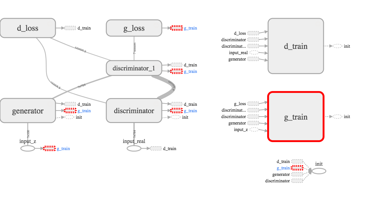
However, it is somewhat misleading. The tensorboard is better at articulate the complicated relationship:
Smiley face
The key point is there are 2 feedback loops. Both give the generator contradicting signal. minimize(g_loss) is trying to make a fake photo as real as possible, so the output logits will be one. One the other hand, minimize(d_loss) is trying to make fake photo stay fake (logits be 0) and real photo stay real (logits be 1).
Put in another word, g_loss gives 100% feedback to the generator, d_loss gives 50% feedback to generator because only half of the loss is from the generator.

Tuesday, June 6, 2017

Deep Learning ND 3b, transfer learning,seq2seq


Recap:

Project: Translation Project

14 Transfer learning

In this lesson, you’ll be using one of these pretrained networks, VGGNet, to classify images of flowers.
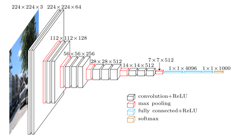
VGG (Visual Geometry Group), is an Oxford team led by Andrew Zisserman and Andrea Vedaldi. In VGGNet, only 3x3 convolution and 2x2 pooling are used throughout the whole network. It is quite famous because not only it works well, but the Oxford team have made the structure and the weights of the trained network freely available online. The Caffe weights are directly downloadable on the project’s web page; there are converted versions for other frameworks available around if you google them. One drawback of VGGNet is that this network is usually big. It contains around 160M parameters. Most of the parameters are consumed in the fc layers.
setup
git clone https://github.com/udacity/deep-learning.git
20170401
cd 20170401/transfer-learning
git clone https://github.com/machrisaa/tensorflow-vgg.git tensorflow_vgg
source activate py3
pip install tqdm
conda install scikit-image
“Transfer_Learning.ipynb” relies on tensorflow_vgg. Running the first code cell will download the parameter file (vgg16.npy, 553MB, ) from aws to the tensorflow_vgg folder.
This notebook is converted from the TensorFlow inception tutorial and shared the same dataset (flow_photos.tar.gz, 229MB). There are five classes: daisy (634 jpg files), dandelion (899), roses(642), sunflowers(700), tulips (800). A total of 3670 instances.
The complete VGGNet is 5 conv layers + 2 dense layers. Here, we only use the output of first 5 conv layers as a feature extractor. the input images have shape (244,244,3). vgg16.Vgg16().relu6 acts as a superpower image preprocessing machine that crush each image into fundamental pieces that are “really” ready for efficient classification. What exactly are these fundamental pieces? Maybe dots, lines, shapes, etc, we are not sure yet.
Supress warning by import warnings
warnings.filterwarnings("ignore") After my 2013 macbook painstakingly spinning for 6785s, I get these exciting pieces named as “codes“(60 MB). Each image or code is a vector with 4096 dimensions.
Then use a simple neural network with a 256-node layer to build a classifier. Train it and store it. Then randomly pick a flower image and let the fortune teller do the magic!
There are several tricks in vgg16.py to expedite the model building. The pre-trained parameter from vgg16.npy is loaded into Vgg16().data_dict during the class initialization and reset to None after building. It is computational expensive because of the many layers and huge number of parameters.
The filter size is stored by the name of the target layer. Each layer actually has multiple filters.
Smiley face
Smiley face

15 Sequence to Sequence

Instructor: Jay Alammar
Sequence to Sequence, published in 2014 by https://arxiv.org/abs/1409.3215, is one of RNN architectures that maps many to many.
One of the authors, Quoc Le, gave a talk: https://github.com/ematvey/tensorflow-seq2seq-tutorials
Chatbot dataset: Cornel Movie Dialogs Corpus, 200 k conversations from 600 movie scripts.

16 Deep Q learning

use neural networks to replace the Q-table.
gym

Project: language translation

It’s all about getting familiar with the RNN architectures using Tensorflow. The codes are almost identical to Course 15: seq2seq.